Creating, Viewing and Editing Sequences
Creating new sequences
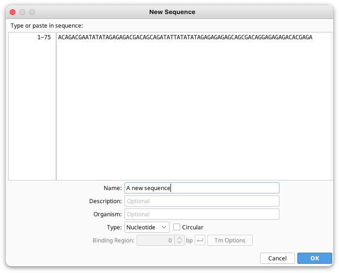
New sequences can be imported from existing files as described in Importing and Exporting Data or they can be created manually by going to Sequence → New Sequence, or File → New → Sequence. Here you can paste or type in the residues for your new sequence, then enter the Name, Description and Organism for your sequence if required. Geneious will automatically determine whether your sequence is nucleotide or protein based on the composition of the bases you enter. You can change this by clicking the Type option. If your sequences are oligonucleotides, choose Primer or Probe as the type. If your primer contains a 5′ extension, you can specify this by setting the length of the binding region. Bases not in the (green) binding region will be included as a 5′ extension.
To create a new sequence from an existing sequence, select the region of sequence that you want then click the Extract button above the sequence viewer, or go to Sequence → Extract Regions. This will create a new sequence document containing the selected sequence.
Sequence lists
Sequence lists make it easier to manage large numbers of sequences by grouping related sequences into a single document. When you import files containing multiple sequences you will be asked if you want to store those sequences in a list. To existing sequences in your database into a list, or combine two lists into one, select the sequences or sequence lists you want to group and go to Sequence → Group Sequences into a List. Note that this copies your sequences into a list and retains the original sequence documents.
To extract sequences from a list, select the sequence(s) you want to extract and go to Sequence → Extract Sequences from List. This will copy each sequence out of the list into a separate document, while retaining the original sequence within the list. To remove a sequence from a list entirely, select it and click the Delete button on your keyboard, or go to Delete under the Edit menu.
The Sequence Viewer
Sequences are displayed in the viewer below the document table. Annotations, translations and analysis graphs are also displayed in this viewer.
Zoom level
Controls for zooming in and out on sequences are located at the top of the side panel, to the right of the sequence viewer. The plus and minus buttons increase and decrease the magnification of the sequence by 50%, or by 30% if the magnification is already above 50%. To zoom in or out by a smaller amount, hold down the alt and/or shift key while clicking the plus or minus button.
 zooms in to fit the selected region in the available viewing area.
 zooms to 100%. The 100% zoom level allows for comfortable reading of the sequence.
 zooms out so as to fit the entire sequence in the available viewing area.
Zooming can also be quickly achieved by holding down the zoom modifier key, which is the Ctrl key on Windows/Linux or the Alt/Option key on Mac OS X, and clicking as described below. When the zoom key is pressed a magnifying glass mouse cursor will be displayed.
-
Hold the zoom key and left click on the sequence to zoom in.
-
Hold the zoom key and Shift key to zoom out.
-
Hold the zoom key and turn the scroll wheel on your mouse (if you have one) to zoom in and out.
-
Hold the zoom key and click on an annotation to zoom to that annotation
You can also pan in the Sequence View by holding Ctrl+Alt (command+Alt on Mac OS X) and clicking on the sequence and dragging.
Selecting part of a sequence
Within the sequence viewer, there are several ways to select part of a sequence, or select a subset of sequences from a list, alignment or assembly:
-
Mouse dragging: Click and hold down the left mouse button at the start position, and drag to the end position. You can modify the boundaries of a selected sequence by holding your mouse over the end of selected region until the <->arrow appears, then clicking and dragging again to select more or fewer bases. To select multiple regions of a sequence or alignment, use the Ctrl (Windows/Linux) or command (Mac) keys.
-
Select from annotations: When annotations are available, click on any annotation to select the annotated residues. As with mouse dragging, multiple selections are supported.
-
Click on sequence name: This will select the whole sequence.
-
Select all: Use the keyboard shortcut Ctrl+A (command+A on Mac) to select everything in the panel.
Keyboard shortcuts for selection of sequences:
-
To quickly select a single residue, double-click on it.
-
To select a block of residues within a single sequence, triple click.
-
To select a block of residues across multiple sequences, quadruple click.
-
To select a block of 10 residues, hold down Shift and Cntrl (alt/option on a Mac) and press the keyboard arrow.
-
To select a specific region of sequence, click at beginning of the region you want to select, hold down Shift and then click the end.
-
To modify the right-hand end of a selection, hold down Shift/alt (command on a Mac) and use the right/left arrows to select more or fewer bases. Holding down Shift and Cntrl (alt/option on a Mac) modifies the selection by 10 bases at a time.
-
To select the same region across multiple sequences in an alignment, select the region you want in the first sequence, then hold down Shift / alt (command on a mac) and click the down arrow to apply the selection to the sequences underneath. Holding down Shift /Cntrl (alt/option on a mac) while pressing the down arrow will select the sequences in batches of 10.
Go to position
To jump to a particular base in a sequence you can use  Go to base under the Edit menu (for amino acid sequences, this appears as Go to Residue). This allows for the instant navigation to a particular nucleotide or amino acid coordinate for any sequence in the current document selection. It also allows the selection of a particular region of sequence, either for individual sequences or across sequence lists and alignments, or the selection of particular sequences out of a sequence list. Formatting examples are given in the setup dialog. Go to Position also appears next to the sequence viewer when in genome view
Circular sequences
When a circular sequence is selected, the default view is to display the sequence as circular. The view can be rotated by using the scrollbar at the bottom or by turning the mouse wheel. Even though a sequence is circular, you can display it as a linear sequence using the Linear view checkbox under the  General section.
To change a linear sequence into a circular sequence, select the sequence then go to Sequence → Circular Sequence, then click Save. This will join the ends of your sequence up to create a circular sequence, but does not check for overlapping ends. Circularization will affect how some operations (such as restriction digest and map to reference) deal with the sequences.
To show a fully zoomed out circular overview next to the zoomed in view of a sequence, use the Circular Overview checkbox under the General section.
The circular overview displays a green box to indicate the region currently visible in the zoomed in view on the right. All settings in the controls (apart from the types of annotations to show) have no effect on the circular overview.
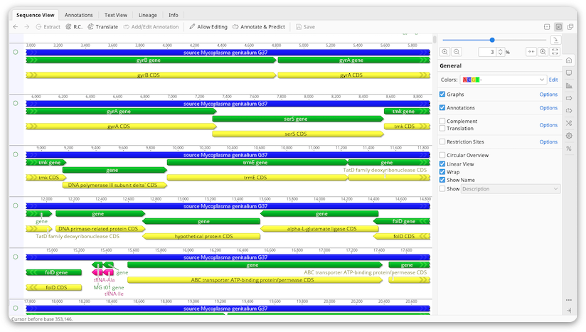
Genome View
The genome view is displayed when sequences larger than 100,000 bp are selected (either as individual sequences or within a sequence list).

The genome viewer contains additional controls which allow for the efficient navigation of large sequences:
1. The Go to Position button allows for the instant navigation to a particular nucleotide coordinate for any sequence in the current document selection. It also allows the selection of a particular region of sequence, or the selection of particular sequences out of a sequence list.
2. A minimap is shown above the sequence viewer which shows a representation of the entire sequence plus its underlying annotations. The portion of the sequence currently visible in the viewing window is highlighted with a green box on the minimap, showing the relative position of the visible section to the overall sequence.
The minimap can also be used to quickly navigate around the visible sequence. Clicking on a section of the minimap will jump the sequence viewer to center on that position. Double-clicking the minimap will zoom further in on the clicked section. Finally, highlighting a section of the minimap using a click-drag-release action will display the highlighted region in the sequence viewer.
The Side Panel Controls
The panel to the right of the sequence viewer allows you to control what is displayed in the sequence viewer (e.g. translations, consensus sequences, graphs and annotations), displays sequence statistics, and provides functions for finding annotations, ORFs, and restriction sites on your sequences. A brief description of each tab is given below:
General Options
Contains the color options, check-boxes to turn on and off main aspects of the sequence view and options for what to display as the name of each sequence.
 Display
Contains options for displaying the translation and/or complement of a sequence, and turning off the original nucleotide sequence. This tab is not displayed for protein sequences.
 Graphs
This option is visible when viewing nucleotide or protein sequences, chromatogram traces, sequence alignments or assemblies, and includes graphs for GC content, Identity, Coverage, and Quality. The graphs available for display depend on the type of sequence you are viewing. For more details see nucleotide and protein graphs and alignment and contig graphs.
 Annotations
On sequences containing annotations this tab will show a yellow arrow. It contains controls for turning on and off annotations of each type, customising the way each type is displayed, and filtering based on annotation name or type. For more information see working with annotations.
 Live Annotate and Predict
Contains real-time annotation generators such as Annotate from Database, Find ORFs and Transfer Annotations. To use one of these, turn on the check-box at the top of the generator you want to use and annotations will immediately be added to the sequence. You can then change settings for the generator and the annotations will change on the sequence in real-time as you do. If you want to save the annotations permanently on the sequence click Apply.
 Restriction Analysis
This behaves similarly to the Live Annotate & Predict section above. For more information see Cloning.
 Advanced
Contains advanced options for controlling the look of sequences and alignments, including wrapping, numbering, annotation placement and font sizes. See Advanced Sequence View options.
 Statistics
Displays statistics about the sequence or alignment currently being viewed, such as length, molecular weight and nucleotide, codon and amino acid frequencies. See Statistics for more information.
Sequence Colors
The colors of nucleotide and amino acid sequences can be set under the General Options tab by clicking the drop down menu next to Colors.
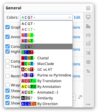
Coloring schemes differ depending on the type of sequence. For example, the Polarity and Hydrophobicity color schemes are available only for protein sequences. Alignments and assemblies can be colored by similarity, read direction and paired distance (if paired reads are used), in addition to standard options.
To change the colors that a particular color scheme uses, click the Edit button then click each base and select the new color you wish to use.
Similarity Color Scheme
The similarity scheme is used for quickly identifying regions of high similarity in an alignment.
In order for a column to be rendered black (100% similar) all pairs of sites in the column must have a score (according to the specified score matrix) equal to or exceeding the specified threshold.
So for example, if you have a column consisting of only K (Lysine) and R (Arginine) and are using the Blosum62 score matrix with a threshold of 1, then this column will be colored entirely black because the Blosum62 score matrix has a value of 2 for K vs R.
If you raised the threshold to 3, then this column would no longer be considered 100% similar. If the column consisted of 9 K's and 1 R, then continuing with the threshold value of 3, the 9 K's which make up 90% of the column would now be colored the dark-grey (80%→100%) range while the single R would remain uncolored.
If instead the column consisted of 7 K's and 3 R's (still with threshold 3) then 70% of the column is now similar so those 7 K's would be colored the lighter grey (60%→80%) range.
Alternatively, going back to the default threshold value of 1, and with a column consisting of 7 K's, 2 R's and 1 Y, now since the 7 K's and 2 R's have similarity exceeding the threshold whereas the Y is not that similar to K and R, the K's and R's will be colored dark grey since they make up 90% of the column.
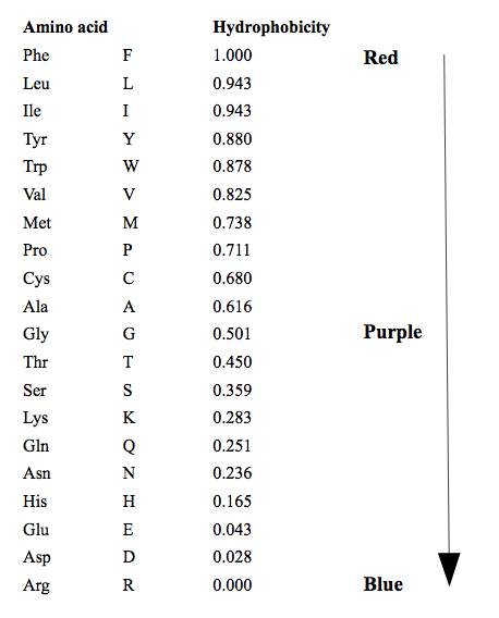
Hydrophobicity color scheme
This colors amino acids from red through to blue according to their hydrophobicity value, where red is the most hydrophobic and blue is the most hydrophilic. The values the color scale is based on are shown below. These values are taken from https://web.expasy.org/protscale/pscale/Hphob.Black.html
Polarity color scheme
This colors amino acids according to their polarity as follows:
Yellow: Non-polar (G, A, V, L, I, F, W, M, P) Green: Polar, uncharged (S, T, C, Y, N, Q) Red: Polar, acidic (D, E) Blue: Polar, basic (K, R, H)
Graphs
The  Graphs tab enables you to display a range of additional metrics on your sequences. The type of graphs which are available depend on the type of sequence you are viewing, and are listed in the sections below. For information on alignment graphs, see Alignment viewer graphs. The number control to the right of each graph controls the height of that graph (in pixels).
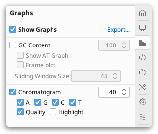
Sliding window size. Many types of graph use a sliding window when calculating values. This calculates the value of the graph at each position by averaging across a number of surrounding positions. When the value is 1, no averaging is performed. When the value is 3, the value of the graph is the average of the residue value at that position and the values on either side.
The numerical values of the graphs can be exported in csv or wig format by clicking the Export button in the Graphs tab, or by going File → Export → Graphs.
Nucleotide sequence graphs
GC content. This plots a graph of the GC content of the sequence within a window of specified length as the window is moved along the sequence. If Frame Plot is checked, the graph shows the GC content in the 3rd codon position only for each frame, where frame 1 = red, frame 2 = green and frame 3 = blue.
Chromatogram. This is available with chromatogram traces, and displays the chromatogram trace above the sequence. If Qual is checked the quality scores are displayed as a blue graph overlaid on the chromatogram.
Protein sequence graphs
Amino Acid Charge. This runs the EMBOSS charge tool to plot a graph of the charges of the amino acids within a window of specified length as the window is moved along the sequence.
Hydrophobicity. This displays the Hydrophobicity of the residue at every position, or the average Hydrophobicity when there are multiple sequences.
pI. pI stands for Isoelectric point and refers to the pH at which a molecule carries no net electrical charge. The pI plot displays the pI of the protein at every position along the sequence, or the average pI when multiple sequences are being viewed. The values in this graph are normalised such that the amino acid with the lowest PI has a value of 0, and the amino acid with the highest PI has a value of 1, and all other amino acid's values are interpolated linearly according to their PI.
Advanced sequence view options
Advanced options for controlling the look of sequences and alignments are under the  Advanced tab. These options are as follows:
Layout:
-
Wrap sequence. This wraps the sequences in the viewing area.
-
Linear view on circular sequences. This forces circular sequences to be shown linearly.
-
Spaces every 10 bases. If you are zoomed in far enough to be able to see individual residues, then an extra white space can be seen every 10 (or whatever number you choose) residues when this option is selected.
Properties
-
Numbering. Enables the display of base position number above the sequence residues. For alignments and assemblies, options are available for displaying the numbering of consensus, reference, alignment and/or all original sequences.
-
Mini-map. Enables the display of a mini-map at the top of the sequence viewer which highlights the currently displayed location in the entire sequence.
-
Outline residues when zoomed out. This adds a fine line around the sequence which can help with clarity and printing.
Annotations
-
Labels. This option changes where the labels are displayed on the annotation: "Inside", "Outside", "Inside or Outside" and "None".
-
Overlay when zoomed out. When only a single annotation covers a region, it will be placed on top of the sequence.
-
Compress annotations. This option reduces the vertical height of the annotations on display. This reduces the space occupied by annotations by allowing them to overlap and increases the amount of the sequence displayed on the screen.
-
Show arrow tips. Displays the directional indicator for an annotation as a large arrow tip.
-
Hide excessive labels. This will reduce screen clutter by removing annotation labels which are too frequent.
Sizes
Here you can set the font size for bases, labels, names and numbering.
Statistics
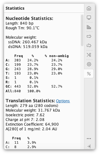
The  Statistics tab displays statistics about the sequence(s) being viewed. If only part of the sequence/alignment or assembly is selected then the statistics displayed will correspond to the highlighted part. The length and number of sequences currently selected is shown at the top of the Statistics tab.
Several of the metrics displayed in the Statistics tab can also be displayed as columns in the document table. These include sequence length, % pairwise identity, % identical sites, mean coverage, molecular weight and several protein statistics such as extinction coefficient and isoelectric point. The value in the document table will be for the entire document, not the currently selected region.
Molecular weight and protein statistics were added to the document table in Prime 2021, and will not appear in the table for documents created in an earlier version of Geneious unless that document is edited in Prime 2021. If you wish to add these statistics to the document table for documents created in earlier versions of Geneious, select the folder containing the document and go to Tools → Preferences → Appearance and Behavior and select Recalculate statistics now. Note that for performance reasons these statistics are only calculated on documents comprised of less than 10,000 bp or aa (this threshold applies to the total number of residues and gaps over all sequences in a document).
General statistics
-
Residue frequencies: This section lists the residues and their frequencies for both DNA and amino acid sequences, for both single sequences and alignments/assemblies. It gives the frequency of each nucleotide or amino acid over the entire length of the sequence, including gaps. If there are gaps, then a second percentage frequency is calculated ignoring gap characters. The G+C content for nucleotide sequences is shown as well for easy reference (see GC content, below).
-
Amino acid and codon frequencies: These are listed for nucleotide sequences based on the current translation options. Click Options to change the translation options. For codon usage statistics, the frequency of all 64 codons (with their associated amino acid) will be displayed. If any CDS contains non-standard start codons then some of the 64 codons may be split into 2 entries based on whether they translate to methionine or their standard translation.
-
Amino acid group frequencies: This section list the frequencies of certain types of amino acids as groups. Total frequencies and percentage frequencies of non-gap, non-ambiguous amino acids are given for Acidic (DE), Basic (RHK), Charged (DERHK), Polar Uncharged (NCQSTYW), Hydrophobic (AGILMPVFW), GC-rich (GARP), and AT-rich (FINKY) groups. These groupings were taken from Biochemistry 8th Edition (Berg, Tymoczko, Gatto, and Stryer).
-
Rough Tm: A rough calculation of the melting point for a nucleotide sequence using the following calculations:
If the sequence is less than 14bp in length (Marmur and Doty 1962):
Rough Tm = 4 x GC count + 2 x AT count
If the sequence is greater than 13bp in length (Chester and Marshak 1993):
Rough Tm = 69.3 + (0.41 x %GC) - (650/length)
-
Molecular Weight: For protein sequences, the following values are used for the amino acids:
A=71.0788 R=156.1875 N=114.1038 D=115.0886 C=103.1388 E=129.1155 Q=128.1307 G=57.0519 H=137.1411 I=113.1594 L=113.1594 K=128.1741 M=131.1926 F=147.1766 P=97.1167 S=87.0782 T=101.1051 W=186.2132 Y=163.1760 V=99.1326 U=150.0388 O=237.3018
For DNA sequences, the following values are used:
A=313.21 T=304.2 G=329.21 C=289.18
The DNA molecular weight assumes no modification of the terminal groups of the sequence.
If the sequence is a single-stranded, synthesised oligonucleotide (e.g. by primer extension), the value is adjusted for the removed phosphate group by using:
Molecular Weight = calculated molecular weight - 61.96
If the sequence is a single-stranded sequence cut by a restriction enzyme, the value is adjusted for the extra 5′-monophosphate left by most restriction enzymes by using:
Molecular Weight = calculated molecular weight - 61.96 + 79.0
For dsDNA, these values are adjusted for both strands.
For RNA sequences, the following values are used:
A=329.21 U=306.2 G=345.21 C=305.18
The RNA molecular weight assumes no modification of the terminal groups of the sequence. For a 5′-triphosphate group, weights are adjusted using
Molecular Weight = calculated molecular weight + 159.0
-
Isoelectric Point: Calculates the isoelectric point of a protein using the bisection method described at isoelectric.org. Amino acid pKa values were taken from the CRC Handbook of Chemistry and Physics 90th Edition, with general pKa values for terminal amino and carboxy groups taken from Biochemistry 8th Edition (Berg, Tymoczko, Gatto, and Stryer).
-
Charge at pH 7: Estimates the overall charge of a protein at pH 7.0 using methods described at isoelectric.org. Amino acid pKa values were taken from the CRC Handbook of Chemistry and Physics 90th Edition, with general pKa values for terminal amino and carboxy groups taken from Biochemistry 8th Edition (Berg, Tymoczko, Gatto, and Stryer).
-
Extinction Coefficient: Calculates the extinction coefficient of a protein as per Gill and Hippel, 1989, using the following values for the amino acids and assuming all cysteines are paired in a disulfide bridge (making cystine): C=62.5 (only counting up to an even number) W=5500 Y=1490
-
A[280] of 1 mg/ml: The correction factor at 280nm, calculated by dividing the extinction coefficient by the molecular weight.
Statistics for multiple sequences (lists, alignments, assemblies)
-
Sequences: The number of sequences in the document, or in the currently selected region.
-
Identical sites: When viewing alignments or assemblies this considers only those columns in the alignment that have at least 2 nucleotides/amino acids/gaps that are not free end gaps and are not columns consisting entirely of gaps. A column not meeting this requirement is not even counted as non-identical for the percentage calculation. A column meeting this requirement is considered identical if it contains no internal gaps and all the nucleotides/amino acids are identical. Ambiguity characters are not interpreted, so a nucleotide column of A and R is not considered identical.
-
Pairwise % Identity: When viewing alignments or assemblies this gives the average percent identity over the alignment. This is computed by looking at all pairs of bases at the same column and scoring a hit (one) when they are identical, divided by the total number of pairs. Ambiguity characters are interpreted, meaning a nucleotide A vs a nucleotide R is considered to have 50% identity.
For both Identical sites and Pairwise % Identity, the statistics are calculated from the subset of sequences and nucleotides/amino acids selected. If just a single sequence is selected, the statistics are calculated as if all sequences are selected over the selected columns. The consensus sequence is always excluded from calculation of both of these values.
-
Coverage of Bases: When viewing a contig assembly this gives the mean, standard deviation, minimum and maximum of the coverage of each base in the consensus sequence. For small contigs the coverage is further broken down into coverage by reads mapped to the forward and reverse strands. For large contigs, separate forward/reverse coverage can't be efficiently calculated, so is displayed as ?. If your contig has a reference sequence, then the percentage of the ungapped reference sequence that is covered by at least 1 read is also displayed.
Selecting a sub-region of your contig will display statistics for just that region, including calculation of separate forward/reverse coverage on large contigs.
For contigs where reads extend outside the bounds of the reference sequence, the document table mean coverage is calculated excluding regions outside the reference sequence. The mean coverage displayed in the contig viewer statistics in this same situation when nothing is selected includes regions outside the reference sequence. Click on the name of the reference sequence to select just that region in order to display detailed coverage statistics over just the region spanned by the reference sequence.
-
[Ungapped] Lengths of Sequences: Displays the mean, standard deviation, minimum and maximum of the lengths of the sequences.
-
Confidence (mean): When viewing sequences containing quality scores (e.g. chromatograms or NGS reads) this gives the mean of the confidence scores for the currently selected base calls. Confidence scores are provided by the base calling program (not Geneious) and give a measure of quality (higher means a base call is more likely to be correct). An untrimmed value is also displayed if the selected region contains trims.
-
Expected Errors: When viewing sequences containing quality scores, this gives the approximate number of errors that are statistically expected in the currently selected region. This is calculated by converting the confidence score for each base call to the error probability using the formula 10(-Q/10). For example, a base with a quality score of 30 will have an error probability of 0.001. The expected errors value is then calculated by summing up the error rates for each base. This also has a value for the untrimmed selection if the region contains trims.
GC content
For documents that are created or modified in Geneious 8.1 or later, the GC content can also be viewed in the %GC column in the document table.
The %GC column shows the percentage of A, C, G, T, U, S, W nucleotides that are either G, C, or S. Ambiguous bases that contain a mixture of GC and non-GC bases (e.g. R, Y, M, K) are excluded from the calculation. This field is available on all nucleotide sequences, contigs, alignments, and sequence lists that were created or had their sequences last modified in Geneious 8.1 or later. For contigs and alignments, the consensus sequence and reference sequence (if any) are excluded from the calculation.
For sequences within an alignment, contig or list, the %GC column only shows the overall value for the alignment. To see a table of GC percentages for all individual sequences within an alignment or contig, the sequences need to be extracted to stand-alone sequences. Alternatively, individual values can be viewed in the statistics panel by clicking on the name of the sequence to select it.
Sequences in a list or alignment can be sorted by GC content by right clicking in the sequence viewer and choosing Sort → %GC.
Customizable text view for sequences
In Geneious Prime 2019.1 onwards, the Text View tab is able to display sequences or alignments in a customisable rich text or plain text document, which can then be exported or copied and pasted into a text or Microsoft Word document. Sequences can be displayed in either Genbank format, or in a custom format where the user can choose the layout and add coloring and highlighting. For further information on the options available, please see this post on our knowledge base.
Editing sequences
To edit sequence(s) or an alignment click the Allow Editing toolbar button.
You can manually enter or delete sequence, or use any of the standard editing operations, such as Copy (Ctrl/command+C), Cut (Ctrl/command+X), Paste (Ctrl/command+V), Paste Without Annotations (Shift+Ctrl/command+V), Paste Reverse Complement and Undo (Ctrl/command+Z). All operations are under the main Edit menu, or can be accessed by right-clicking in the sequence view and selecting the option from the popup window.
To insert sequence, click at the position where you want to insert the sequence and type or paste it in. Normally existing residues will be shifted to the right when you insert sequence; to get them to shift to the left hold down the Shift key as you insert the sequence. To overwrite sequence, select the sequence you wish to overwrite and type or paste the new sequence in.
To select sequences or regions of sequence, there are several options:
-
To quickly select a single residue, double-click on it.
-
To select a block of residues within a single sequence, triple click.
-
To select a block of residues across multiple sequences, quadruple click.
-
To select a block of 10 residues, hold down Shift and Cntrl (alt/option on a Mac) and press the keyboard arrow.
-
To select a specific region of sequence, click at the beginning of the region you want to select, hold down Shift and then click the end.
-
To select the same region across multiple sequences in an alignment, select the region you want in the first sequence, then hold down Shift / alt (command on a mac) and click the down arrow to apply the selection to the sequences underneath. Holding down Shift /Cntrl (alt/option on a mac) while pressing the down arrow will select the sequences in batches of 10.
Sequences can be reordered within an alignment by clicking the sequence name and dragging.
Sequences can be removed from an alignment by right-clicking (Ctrl+click on Mac OS X) on the sequence name and choosing the remove sequence option. Alternatively, select the entire sequence (by clicking on the sequence name) and press the delete key.
To delete a region of a sequence or alignment, select the region and press the delete or backspace key. Normally this will move residues on the right into the deleted area. To move the residues on the left into the deleted area, hold down the Shift key while deleting.
To drag a sequence to the left or right, select the region you want to move, then click it again and drag it to the position you want. Dragging will either move residues over existing gaps or open new gaps when necessary. Dragging a selection consisting entirely of gaps moves the gaps to the new location.
After editing is complete, click Save to permanently save the new contents.
Changing the numbering of your sequence
To change the base numbering on a sequence, go to Sequence → Change Residue Numbering. On a circular sequence this function can be used to shift the origin of the sequence to a different location. On a linear sequence this can be used to indicate that the sequence is a subsequence of a larger sequence; to number a sequence with respect to a particular location (ie make the start of a gene base 1); or to reverse the numbering of a sequence. This will introduce two numbering systems into your sequence: the original numbering (Standard), and the numbering that you have specified (Source). To choose which numbering is displayed on your sequence, go to the Advanced settings tab choose the numbering option you want under Properties.
Convert between DNA and RNA
This option is under the Sequence menu, and changes all T's in a sequence to U's or vice versa, depending on the type of the selected sequence. Once this is performed, click "Save" in the Sequence View to make the change permanent.
Concatenating sequences
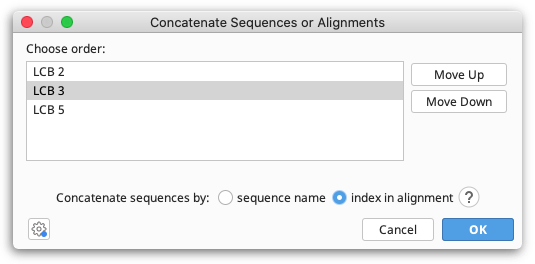
To join several sequences end-on-end, select all the sequences and go to Tools → Concatenate Sequences or Alignments. This creates a single sequence document from the input sequences. The order in which sequences are concatenated can be chosen in the setup dialog box, and the resulting sequence can be circularized if required by checking Circularize sequences. If one or more of the component sequences was an extraction from over the origin of a circular sequence, you can choose to use the numbering from that sequence, thus producing a circular sequence with its origin in the same place as the original circular sequence. Overhangs will be taken into account when concatenating.
You can also concatenate sequence list or alignment documents. When you concatenate multiple sequence lists or alignments, sequences from each input document will be matched by either name or index and concatenated.
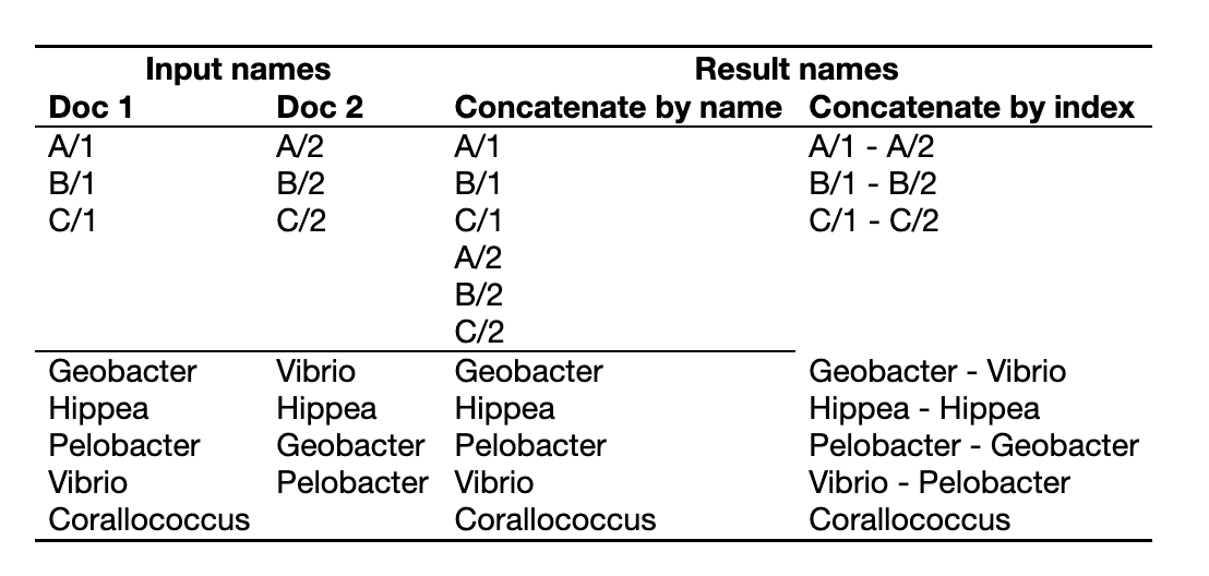
Concatenating by name allows you to match sequences in different alignments or sequence lists that aren't in the same order. To concatenate by name, sequences to be concatenated must have exactly the same name, including any spaces or punctuation. Note that names are case sensitive: H. sapiens and H. Sapiens are considered to be different. The one exception to this rule is that the special suffices "extraction" and "(reversed)" are ignored.
Concatenating by index allows you to match sequences based on their order in lists or alignments, even if they don't have the same names. The first sequence across all lists will be concatenated together, as will the second and so on. This can be very useful when you have additional information appended to your sequence names, such as sequencing read direction or gene names or accession numbers. You can change the sort order for a list of sequences prior to concatenating by right clicking on the sequence names and selecting one of the Sort submenu options.
The number of sequences in the set of alignments or sequence lists you wish to concatenate can be different; however, if you concatenate by index and sequences from the middle of the list are missing in some documents, later sequences will be concatenated with the wrong partners.
| If you have... | You should concatenate by: |
|---|---|
| Sequences in arbitrary order, but matching sequences have the same names | Name |
| Sequences in fixed order, but matching sequences have different names | Index |
| Sequences in fixed order, matching sequences have the same names | Name or Index |
| Sequences in arbitrary order, matching sequences have different names | Sort or rename sequences before concatenating (see Batch Rename) |
Examples: Concatenating by Name vs. Index
Complement and Reverse Complement
To display the complement (3′ to 5′) of a sequence (displayed 5′ to 3′), check the Complement box in the  Display tab. Note that the complement option is for display purposes only, you cannot select or edit the complement sequence. If you wish to create a separate document to work with the complement (not reverse complement) of a sequence, you will need to install the Complement or Reverse plugin by going to Tools → Plugins. Once the plugin is installed, go to Sequence → Complement only to create a new document containing the complement.
To reverse complement a nucleotide sequence (i.e. reverse the sequence direction and replace each base by its complement), click the R.C button above the sequence viewer, or go to Reverse Complement under the Sequence menu. You can also access this option right-clicking in the sequence viewer and selecting it from the popup menu. When you click Save after reverse complementing, the tag (reversed) will be added to the sequence name.
When only part of a sequence is selected, you can choose to either reverse-complement only the selected region and extract it to a new sequence document, or reverse complement the entire sequence. On alignment or contig documents you can reverse complement individual sequences within the alignment or assembly by selecting that sequence, and choosing reverse complement selected sequence.
Translating sequences
The protein translation can be viewed alongside the nucleotide sequence by checking the Translation option in the Display tab. Select the genetic code and reading frame(s) you require. You can also choose to translate relative to selection or annotations such as CDS. In an alignment, the sequence frame can be calculated relative to the individual sequences, the alignment, the consensus or a specific reference sequence. On a contig or alignment, the translation can be displayed on the consensus and reference sequence only, or it can be displayed on all sequences.
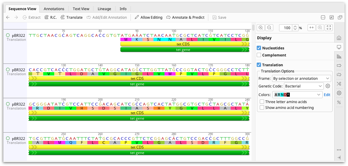
To display the amino acid numbering on the sequence, check the box Show amino acid numbering. The amino acid numbering is displayed below the sequence.
To show three letter rather than single letter amino acids, check the box Three letter amino acids. Translations which have two possibilities will always show as single letter amino acids. e.g. V/M. For stand-alone protein sequences, there is no option whether to show three letter codes or not. Instead, three letter codes are automatically displayed when the zoom level is 200% or higher and when not in editing mode.
If you wish to view only the translation and turn off the nucleotide sequence, uncheck Nucleotides. However, this is only for display purposes: if you wish to work with the translation in downstream analysis you must extract it to a separate document using the Translate button above the sequence viewer. The Translate button will create new protein document from the translated DNA, using your choice of reading frame and genetic code. This option can also be accessed from the Sequence menu.
To copy the translation of a selected region of a nucleotide sequence, right click on the selected sequence and choose Copy Translation from the menu. The copied translation can then be pasted into the New Sequence box or into a document outside of Geneious.
Note: If a CDS annotation contains an internal stop codon, it will be assigned as a premature stop codon and will be represented by an asterisk (*) in the translation view. The CDS after the premature stop codon will appear faded yellow, to represent the truncated protein sequence.

Genetic Codes
Geneious Prime supports a range of genetic codes which can be chosen from the drop-down menu in the Translation options. To set a default genetic code which will apply to all documents in your database, click the Settings cog next to the drop-down menu. You can also enter a custom genetic code here by clicking Add and editing an existing genetic code template.
Back Translating
To create a nucleotide sequence from a protein document, go to Sequence → Back Translate. Ambiguous back-translation uses a specific genetic code to produce a nucleotide sequence with ambiguous bases, so that every possible codon is represented for each amino acid. Un-ambiguous back-translation uses codon usage tables to produce a nucleotide sequence where the most frequently used codon for that organism is used for each amino acid. Codon usage tables for some organisms are provided, or you can you can import custom codon usage tables in GCG CodonFrequency and EMBOSS cusp formats. For further instructions, see How do I create a custom codon usage table?.
Viewing chromatograms
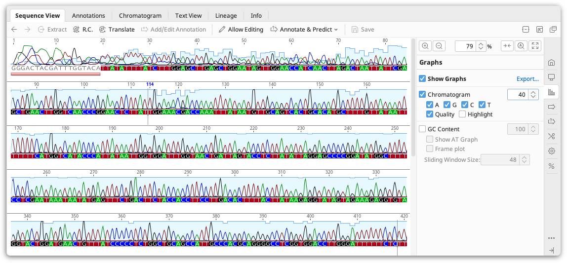
Geneious Prime can view chromatogram information from files imported in .ab1 or .scf format. If the chromatograms are not visible, check Chromatograms under the Graphs tab.
Chromatogram files are produced from sequencing machines such as the Applied Biosystems 3730 DNA analyzer. The raw output of a sequencing machines is known as a trace, a graph showing the concentration of each nucleotide against sequence positions. The raw trace is processed by a "Base Calling" software which detects peaks in the four traces and assigns the most probable base at more or less even intervals. Base calling may also assign a quality measure for each such call, typically in terms of the expected probability of making an erroneous call. Geneious does not perform base-calling itself: this information is already contained in the .ab1 or .scf file.
Chromatogram peaks for individual bases can be turned off by checking the A/G/C/T boxes in the Graphs tab. Note that since the distance between bases as inferred from the trace varies the trace may be either contracted or expanded compared with the raw data. The vertical scale of the chromatogram can be adjusted by clicking and dragging on the graph itself. The total height of the graph can be adjusted by increasing the number displayed next to the graph on the right of the Sequence View.
Quality. The quality scores associated with a chromatogram can be viewed by checking the Qual box under the Chromatogram graph options. This displays a quality measure (typically Phred quality scores) for each base as assessed by the base calling program. The quality is shown as a shaded blue bar graph overlaid on top of the chromatogram. Note that those scores represent an estimate of error probability and are on a logarithmic scale - the highest bar represents a one in a million (10-6) probability of calling error while the middle represents a probability of only a one in a thousand (10-3).
Poor quality regions of the chromatogram can be trimmed using Trim Ends under the Annotate and Predict menu.
Highlighting. When this is turned on, chromatogram peaks that do not match their base call are colored, and all other peaks are greyed out.
To view the raw chromatogram traces, click the Chromatograms tab above the sequence viewer. In this view, the exact location of the base call can be viewed by checking Mark calls. To view sequence logos indicating base quality in this view, check Scale by confidence. The Trace options for X and Y scales allow you to zoom in on the X or Y axes, respectively.
Binning by quality
Chromatograms can be binned on the basis of their quality scores into Low, Medium or High quality bins. The parameters for each of these bins are set under Tools → Preferences → Sequencing - see Configuring sequence binning options for more information). To see the bin for a trace, add the Bin column to the document table by going to View → Table Columns. You can also view the percentage of bases that are low, medium or high quality by adding LQ%, MQ%, and HQ% columns to the document table.
Virtual Gel
The Virtual Gel tab will appear above the sequence viewer when nucleotide documents containing fewer than 50 sequences or 1000 restriction sites are selected.
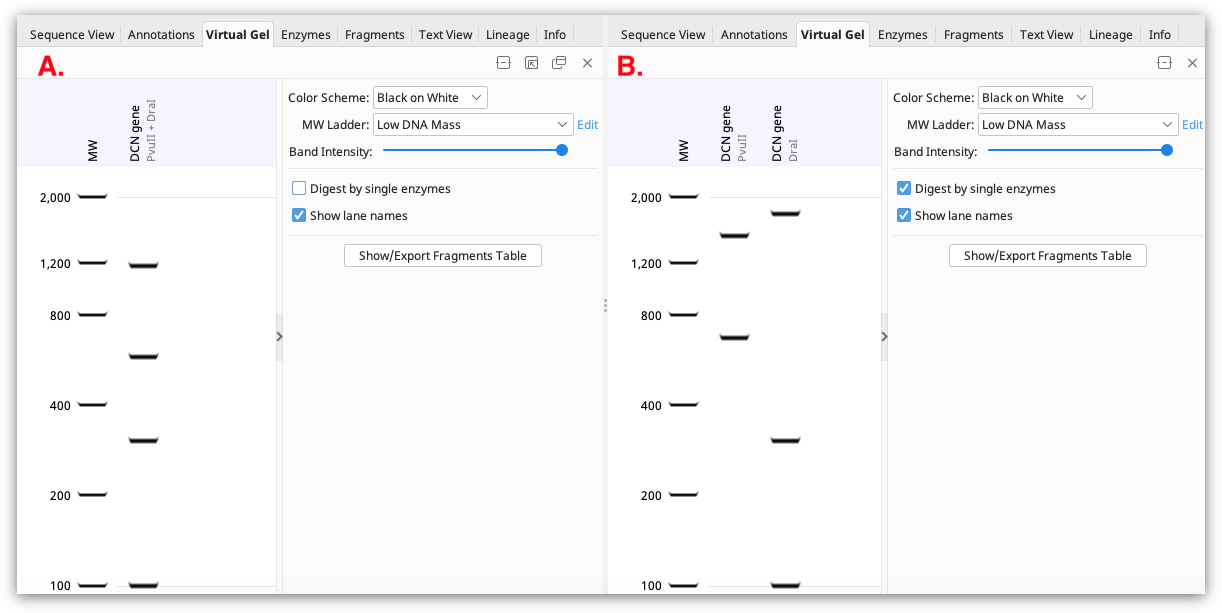
If a single sequence annotated with restriction enzyme sites is selected, the gel displays the fragments that would result from that restriction digest. If the restriction sites are all from a single enzyme, the digest pattern is shown in one lane of the gel. If multiple different restriction enzymes are annotated, the results of digestion with each enzyme will be shown in different lanes if Digest by single enzymes is checked (shown in B below). If this option is unchecked, the result will be shown as a multiple enzyme digest in a single lane (shown in A below).
If multiple sequence documents containing restriction sites are selected (either by bulk-selecting individual sequence documents, or selecting a sequence list), digests for each sequence are shown in separate lanes on the gel (a maximum of 50 sequences can be shown).
The fragment sizes of all bands shown on the gel can be viewed in the Fragments table or by clicking Show/Export Fragments table. This table is only available for sequences with annotated restriction sites.
For sequences which do not have annotated restriction sites, these will be shown in individual lanes on the gel if the sequences are in separate documents, or in one lane of the gel if the sequences are contained in a list (for example the results of the Digest into Fragments operation).
By default, sequences will appear on the gel in the order they are displayed in the document table or sequence list. To change the order of display, simply drag and drop the sequences on the gel to the desired position.
Note that if uncut circular DNA is selected (for example a plasmid sequence with no restriction sites), the band on the gel will show the size of the linear fragment, rather than the supercoiled DNA size. Depending on the size of your DNA and the buffer you use, uncut circular DNA may migrate differently to linear DNA.
Ladders
Geneious contains a built-in list of common ladders which can be selected from the Ladders drop down menu to the right of the viewer. To add another ladder, click Edit next to the Ladders menu, then Edit Ladders File. This brings up a text editor where you can add your ladder to the existing ladders file.
Ladders must be added in the following format:
Name: BP or KBP: fragment sizes separated by commas
For example: 10bp DNA Ladder : BP : 10, 20, 30, 40, 50, 60, 70, 80, 90, 100, 125, 150, 175, 200, 250, 330
Note that fragment sizes must always be listed in base pairs. The designation BP or KBP refers only to the display (KBP looks better for large numbers over 100 kbp). Once you have added the ladder you want, click Save to record the changes.
Meta-data
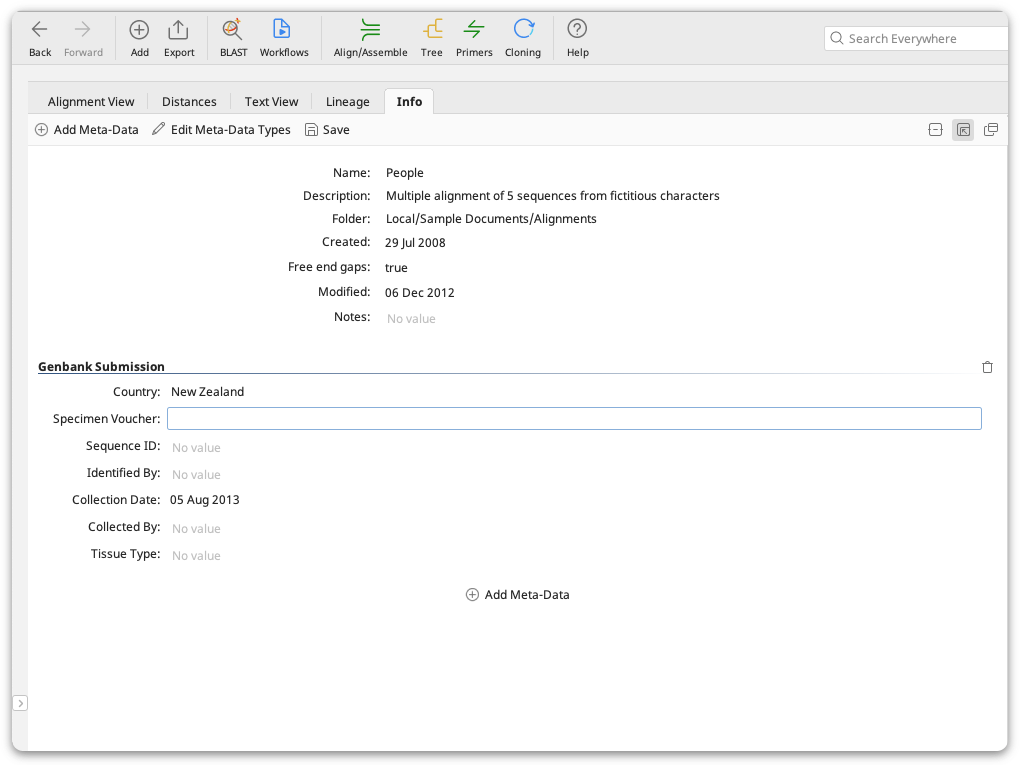
Meta-data is additional information you can add to any of your local documents, for example sample collection history, organism identification, primers used etc. Meta-data is added in the Properties view under the Info tab. This tab displays standard properties of documents such as the name and description, plus any meta-data you have added. Any meta-data that you add can appear in a column in the document table, and can be treated as a user-defined field for use in sorting, searching and filtering your documents.
When multiple documents are selected, the Properties view displays all of the fields and meta-data belonging to the selected documents. When all documents have the same value for a field, it is displayed in the viewer. If the documents have different values, or some of the selected documents do not have a value, then the field will show that it represents multiple values. Changes made to the fields will apply to all selected documents.
You can add meta-data to any of your local documents, including molecular sequences, phylogenetic trees and journal articles. You cannot add meta-data to search results from NCBI or EMBL etc until the documents are copied into one of your local folders.
Adding meta-data
To add meta-data to your document, select the Add Meta-Data button on the toolbar and then choose from the available types. Selecting a meta-data type will create an empty instance of that type. To fill meta-data values just start typing into the fields. See below for information on how to create a new meta-data type.
Editing Meta-Data
To edit existing meta-data fields, simply click on the field and enter your data. Some fields may have constraints (which you can edit in the Edit Meta-Data Types dialog. If the data you have entered does not conform to the constraints of the field, it will be displayed in red and you will be shown the field's constraints in a tooltip.
Tip: To enter a new line in a text field, press Shift+enter or Ctrl+enter**
Creating a new Meta-Data type
Geneious Prime does not restrict you to the meta-data types that it comes with. You can create your own types to store any information you want.
To create a new type, click Edit meta-data types, then click the Create button at the bottom left of the panel. This creates a new type, with one empty field, and displays it in the panel to the right.
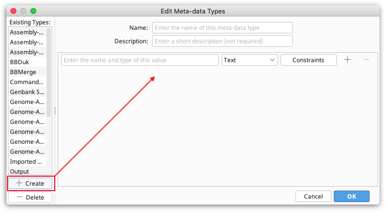
Note. The Name and Description fields distinguish your meta-data type from other user-defined types. They do not have any constraints.
Next, you need to decide what values your Meta-Data Type will store by specifying its fields:
Field name. This defines what the field will be called. It will be displayed alongside columns such as Description and Creation Date in the Documents Table. You can have more than one Field in a single Meta-Data Type - to add or remove a field from the type, click the + or - buttons to the right of the field.
Field type. This describes the kind of information that the column contains such as Text, Integer, and True/False.
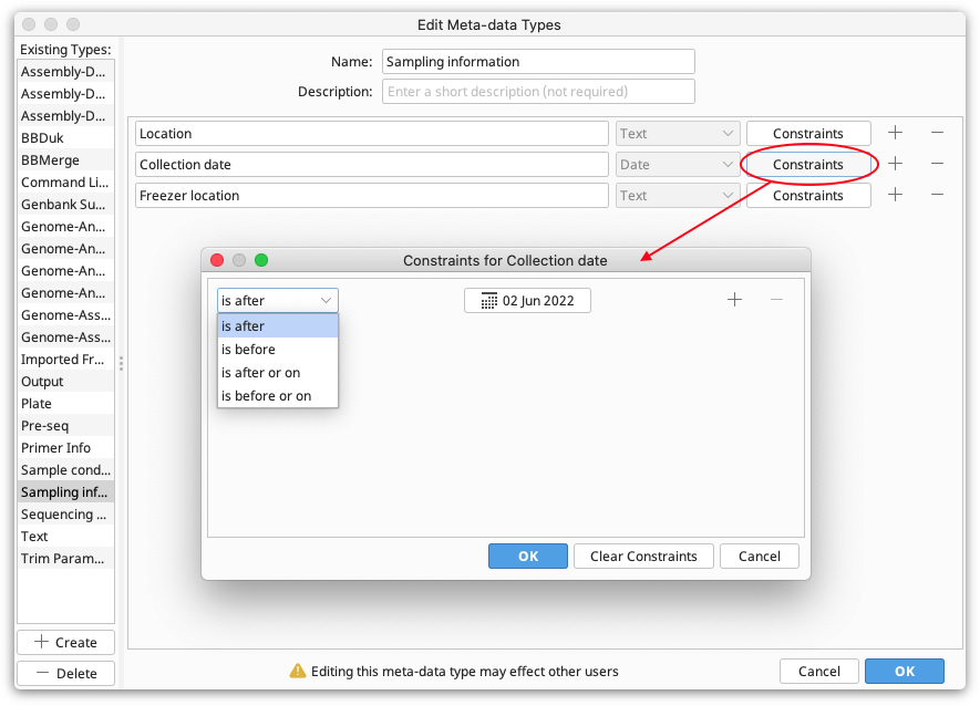
Constraints. These are limiting factors on the data and are specific to each field type. For example, numbers have numerical constraints -- is greater than, is less than, is greater or equal to, and is less or equal to. These can be changed to suit. The constraints for each field can be viewed by clicking the "Constraints" button next to the field. This will show a pop-up menu with the constraints you have chosen.
Editing Meta-Data Types
To edit meta-data types, e.g. by adding and removing fields, click Edit Meta-Data Types. Select the meta-data type you want to edit, and then add, remove or edit the fields as described in Creating a new meta-data type.
Using Meta-Data
The main purpose of meta-data is to add user defined information to Geneious documents. However, meta-data can be searched for and filtered as well. Also, documents can be sorted according to meta-data values.
Searching - Once meta-data is added to a document, it is automatically added to the standard search fields. These are listed under the Advanced Search options in the Document Table. From then on, you can use them to search your Local Documents. If you have more than one Field in a meta-data type, they will all appear as searchable fields in the search criteria.
Filtering - Meta-data values can be used to filter the documents being viewed. To do so, type a value into the Filter Box in the right hand side of the Toolbar. Only matching documents will be shown.
Sorting - Any meta-data fields added to documents will also appear as columns in the Document Table. These new columns can be used to order the table.