Analysis of Assemblies and Alignments

Finding polymorphisms

To easily identify bases which do not match the consensus or reference sequence, turn on Highlighting in the consensus section of the sequence viewer options. Select the options Disagreements to Consensus or Reference depending on your needs. When this is on, matching bases are grayed out and bases not matching are left colored.

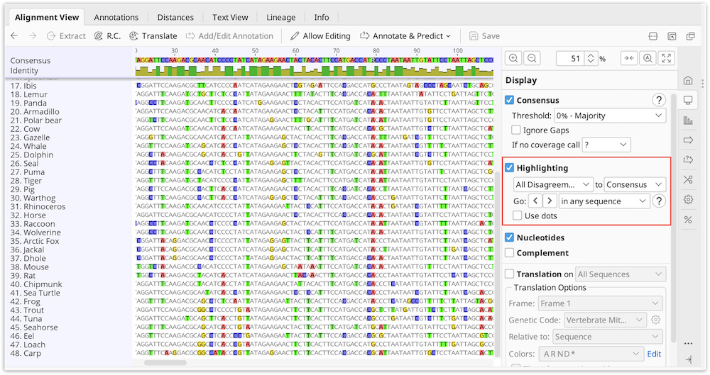
With this on you can quickly jump to each disagreement by pressing Ctrl+D (command+D on Mac OS X) or by clicking the < > arrows in the sequence viewer option panel to the right. Each disagreement can then be examined or resolved.

Find Variations/SNPs

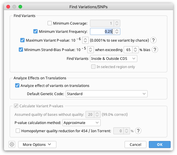
Manually investigating every little disagreement can be time consuming on larger contigs. The Find Variations/SNPs feature from the Annotate & Predict menu will annotate regions of disagreement and can be configured to only find disagreements above a minimum threshold to screen out disagreements due to read errors. This feature can also be configured to only find disagreements in coding regions (if the reference sequence has CDS annotations present) and can analyze the effects of variations on the protein translation to allow you to quickly identify silent or non-silent mutations. It can also calculate p-values for variations and filter only for variations with a specified maximum P-Value.

For full details of how the various settings work in the Variation/SNP finder, hover the mouse over them to read the tooltips or click one of the '?' buttons.

P-values

The p-value represents the probability of a sequencing error resulting in observing bases with at least the given sum of qualities. The lower the p-value, the more likely the variation at the given position represents an real variant. Click the down arrow next to the exponent of the Maximum Variant P-Value setting to increase the number of variants found.

When calculating P-Values:

• The contig is assumed to have been fine tuned around indels
• Ambiguity characters are ignored (other characters in the column are still used)
• Homopolymer region qualities are reduced to be symmetrical across the homopolymer. For example if a series of 6 G's have quality values 37, 31, 23, 15, 7, 2 then these are treated as though they are 2, 7, 15, 15, 7, 2. This is done because variations may be called at either end of the homopolymer and because reads may be from different strands.
• Gaps are assumed to have a quality equal to the minimum quality on either side of them (after adjusting for homopolymers)
• When finding variations relative to a reference sequence, the p-value calculated is for the variant, not the change. In other words the p-values calculated are independent of the reference sequence data.
• The approximate p-value method calculates the p-value by first averaging the qualities of each base equal to the proposed SNP and averaging the qualities of each base not equal to the proposed SNP.

Example: Assume you have a column where the reference sequence is an A and there are 3 reads covering that position. 1 read contains an A in the column and the other 2 reads contain a G. All 3 reads have quality 20 ( = 99% confidence) at this position. We want to calculate the p-value for calling a G SNP in this column.

Since the quality values are all equal, the p-value is the probability of seeing at least 2 G's if there isn't really a variant here. In other words, the probability of seeing 2 G's by chance due to a sequencing error plus the probability of seeing 3 G's by chance due to a sequencing error, which is calculated using the binomial distribution: ³C₂ * 0.01² * 0.99 + ³C₃ * 0.01³ = 0.0003 (^NC_K is a binomial coefficient)

False SNPs due to strand-bias (when sequencing errors tend to occur only on reads in a single direction) can be eliminated by specifying a value for the Minimum Strand-Bias P-value setting. A Strand-Bias P-Value property is added to each SNP to indicate the probability of seeing a strand bias at least this extreme assuming that there is no strand bias. SNPs with a smaller strand bias p-value will be excluded from the results when using this setting.

Strand-Bias >50% P-value example: Assume you have a column covered by 9 reads containing an A, 8 of which are on the forward strand. We calculate the probability of seeing bias at least this extreme, assuming there is no strand-bias, which is the probability of seeing either 0, 1, 8, or 9 reads on the forward strand. Using the binomial distribution, this is ⁹C₀ * 0.5⁹ + ⁹C₁ * 0.5⁹ + ⁹C₈ * 0.5⁹ + ⁹C₉ * 0.5⁹ = 0.039$ ($^NC_K is a binomial coefficient)

Click the up arrow next to the exponent of the Minimum Strand-Bias P-Value setting to increase the number of variants found. If there are any forward/reverse or reverse/forward style paired reads, then variants with strand bias which are less than 1.5 times the insert size from either end of the contig will not be filtered out.

Results display

The results of the Variant/SNP finder are added to the reference sequence in the assembly or alignment as an annotation track. Clicking Save and clicking "Yes" when prompted to apply the changes to the original sequences will add this annotation track onto the original reference sequence file. If there is no reference sequence for the alignment or assembly the annotations are added to the consensus sequence.

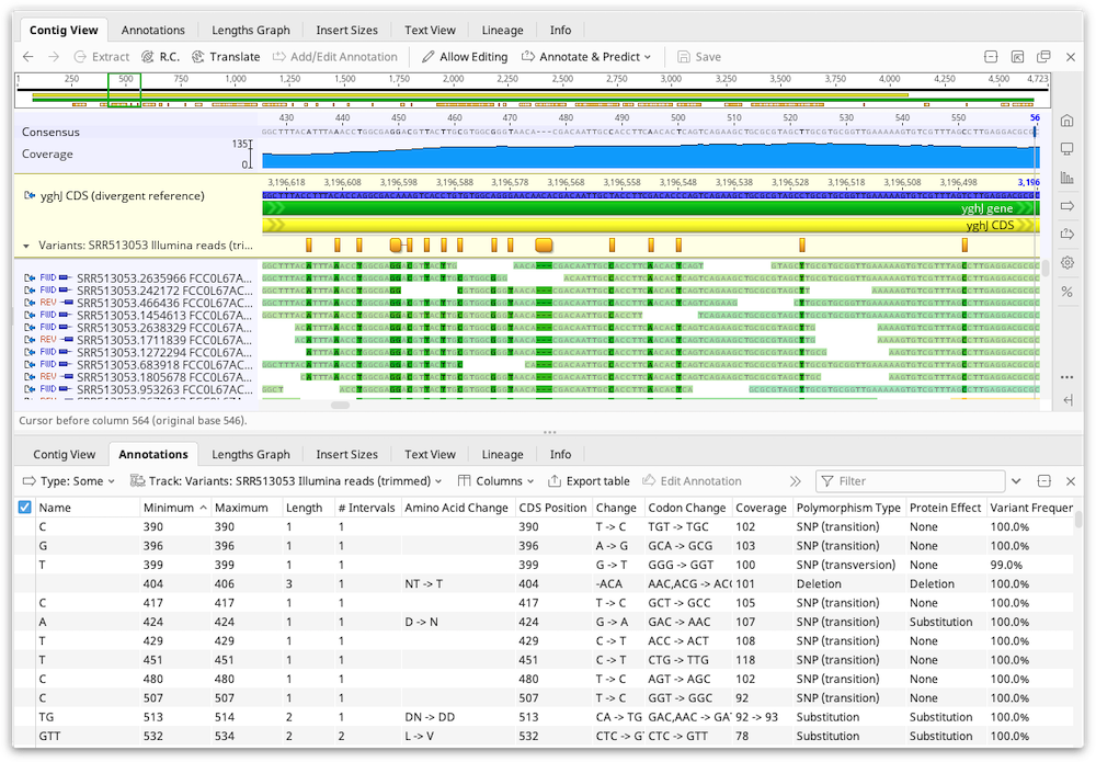
The results are also displayed in the annotations table and the following columns can be displayed:

• Change: Indicates the reference sequence nucleotides followed by the variant nucleotides. For example 'C → A'

• Coverage: The number of reads that cover the SNP region in the contig. The coverage includes both the reads containing the SNP and other reads at that position.

• Reference Frequency: The percentage of reads that agree with the reference sequence at that position. This field will only be present if at least 1 read agrees with the reference sequence.

• Variant Frequency: The percentage of reads that have the variation at that position. For variations that span more than a single nucleotide, the variant frequency may appear as a range (e.g. 47.8% -- 51.7%) to indicate the minimum/maximum variant frequency over that range.

• Polymorphism Type: This may be one of the following.

  SNP (Transition): a single nucleotide transition change from the reference sequence

  SNP (Transversion): a single nucleotide transversion change from the reference sequence

  SNP: At a single position, there are multiple variations from the reference sequence

  Substitution: A change of 2 or more adjacent nucleotides from the reference sequence

  Insertion: 1 or more nucleotides inserted relative to the reference sequence

  Deletion: 1 or more nucleotides deleted relative to the reference sequence

  Mixture: multiple variations from the reference sequence which are not all the same length

For variations inside coding regions (CDS annotations) the following fields can be displayed:

• Codon Change: indicates the change in codon. Essentially this is the same as the 'Change' field, but extended to include the full codon(s). For example 'TTC → TTA'

• Amino Acid Change: indicates the change (if any) in the amino acid(s) by translating the codon change. For example 'F → L'

• Protein Effect: summarizes the change on the protein as either a substitution, frame shift, truncation (stop codon introduced) or extension (stop codon lost)

• Average Quality: is the average of the quality score of all base-calls in reads that have the variation at that position.

Analyzing Expression Levels

Calculating Expression Levels

The Calculate Expression Levels feature from the Annotate & Predict menu calculates normalised expression measures from mapped RNA-seq data.

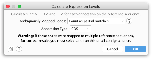
RPKM, FPKM and TPM are calculated for each transcript annotation on the reference sequence of a contig and the results are displayed as a heat map annotation track. Transcript annotations can be of type CDS, Gene, mRNA, miRNA, ncRNA or ORF, and you must specify the annotation type you wish to use when you run Calculate Expression Levels. For simplicity we refer to transcript annotations as CDS annotations for the rest of this section.

If you have multiple reference sequences for each sample (e.g. reads mapped to multiple chromosomes), all contigs from a single sample should be selected and run in a single step.

To calculate differential expression between samples you need to run Calculate Expression Levels on the mapped reads for each sample separately, save the expression level track to the reference sequence, and then compare the results on the reference sequence using Compare Expression Levels.

Counting

The three metrics are calculated by normalizing the count of reads that map to each CDS annotation. If a read at least partially intersects at least one interval from a CDS annotation, then it will be treated as though that read mapped to that CDS annotation.

For reads that map to multiple locations, or reads that map to a location that intersect multiple CDS annotations, these may either be counted as partial matches, excluded from the calculations, or counted as full matches to each location they map to. For example if a read maps to two locations, then it will be counted as if 0.5 reads mapped to each of the two locations.

When calculating statistics, reads that don't map or map outside of an annotation CDS annotation are ignored.

RPKM

Reads per kilobase per million normalizes the raw count by transcript length and sequencing depth.

RPKM = (CDS read count * 10⁹) / (CDS length * total mapped read count)

FPKM

Same as RPKM except if the data is paired then only one of the mates is counted, i.e., fragments are counted rather than reads.

TPM

Transcripts per million (as proposed by Wagner et al 2012) is a modification of RPKM designed to be consistent across samples. It is normalized by total transcript count instead of read count in addition to average read length.

TPM = (CDS read count * mean read length * 10⁶) / (CDS length * total transcript count)

Results

Results are displayed as an annotation track on the reference sequence. By default, annotations are colored based on the TPM property, ranging from blue for 0, through to white for the mean TPM, up to red for the highest TPM for any gene in the sample. In the results view, by clicking on the little down arrow to the left of the track's name, you can choose to color by a different property.

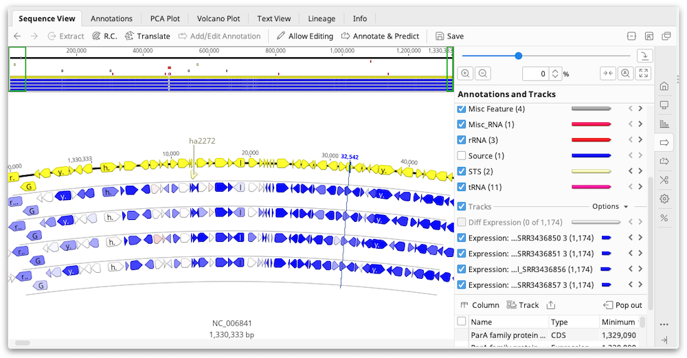
The values for RPKM, FPKM and TPM, as well as the raw read counts, are entered as properties on the annotation and can be displayed by mousing over an annotation. To export these values as a table, switch to the Annotations tab above the sequence viewer then click the Track button and choose the Expression track to display. Then click the Columns button and add the columns for FPKM, RPKM, TPM and/or the raw counts. Once you have the columns you need, you can export the table in .csv format by clicking Export table.

Comparing Expression Levels

Geneious Prime is able to find differentially expressed genes between two or more sample conditions. This can be done through one of two methods: the built-in Geneious method, or the DESeq2 method. The Geneious method should be used when there are two samples only. For more than two samples, the DESeq2 method should be used and requires at least two replicates per condition.

To compare expression levels, you must first assemble the reads for each sample, to the same reference sequence(s), then run Calculate Expression Levels from the Annotate & Predict menu on each contig assembly. This will save an Expression Level track for each contig on the reference sequence(s). To compare these tracks, select the reference sequence document(s) and go to Annotate & Predict → Compare Expression Levels.

If your samples map to multiple reference sequences, you should run both Calculate Expression Levels and Compare Expression Levels on all contigs from a single sample at once to produce correct results in all cases. However, when using the Geneious method, Compare Expression Levels can optionally be run on just one reference sequence at a time when using a normalization system other than Median of Gene Expression Ratios.

Geneious Method for Comparing Expression Levels

The Geneious method should be used to compare expression between two single-sample conditions. Either read counts, fragment counts or transcript counts from each annotation can be compared.

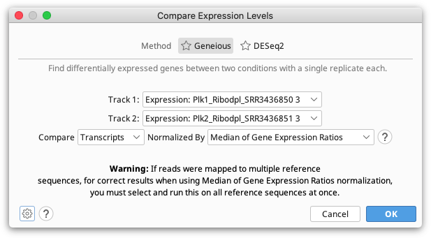
Since a single transcript can produce multiple reads and fragments, the number of reads and fragments produced aren't independent events so the confidence values produced by comparing these are unlikely to be accurate. For this reason we recommend comparing samples using transcript counts.

Normalization

Different samples produce different quantities of transcripts, therefore, in order to compare values between samples, the counts need to be normalized using one of the following methods.

• Total Count: The counts in each gene are scaled according to the total number of transcripts mapped to all genes. For example, if one sample has twice as many transcripts mapped as the other sample, then the counts for each gene need to be halved to make them comparable with the other sample.

• Median Expression: The expression level of all expressed genes from the sample are calculated and the median values of these from each sample are used to normalize. For example, if one sample has a median twice as high as the other sample, then the counts for each gene need to be halved to make them comparable with the other sample.

• Total Count Excluding Upper Quartile: The expression level of all expressed genes from the sample are calculated and the total number of reads, fragments, or transcripts from the lowest 75% of those are totaled. Values are normalized between samples based on this total.

• Median of Gene Expression Ratios: For each gene the ratio of the expression level between samples is calculated. Then the median ratio across all expressed genes is used as the normalization scale. This normalization method is the same as that implemented by DESeq2.

All of these normalization methods (and more) are described and compared by Dillies et al 2012, who recommend using Median of Gene Expression Ratios. One reason for this is that a few highly expressed genes can greatly affect the total number of transcripts produced, so this can distort the fraction of the total reads that contribute to genes with lower expression. The choice of normalization method determines the Differential Expression Ratio for each gene.

P-Value Calculation

In addition to calculating the differential expression ratio, it is useful to know whether or not that differential expression is statistically significant. This is represented by a p-value. A number of advanced methods have been published for the calculation of p-values based on a range of assumptions. Many of these are compared by Soneson & Delorenzi 2013, who conclude that no single method is optimal under all circumstances and that very small samples sizes impose problems for all evaluated methods.

In this basic differential expression plugin in Geneious we have implemented a simple statistical test based on the assumption that the gene which each observed transcript came from is an independent event.

For a given gene, the probability that a randomly selected transcript would come from that gene is calculated as number of transcripts mapped to that gene/total number of transcripts from that sample. This probability is normalized, the mean probability between the two samples calculated, and this mean un-normalized for each sample. This produces an expected probability that a randomly selected transcript from this sample comes from that gene, assuming that this gene is not differentially expressed.

The Binomial Distribution is used to calculate the probability that an observed count at least as extreme as the observed one would be seen, assuming this non-differentially expressed mean probability. The probabilities from each sample are multiplied together to form the p-value.

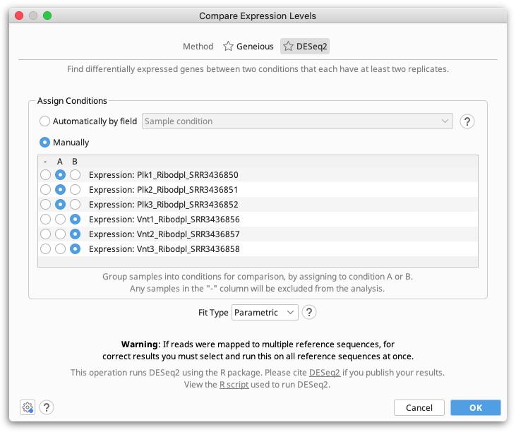
DESeq2 Method for Comparing Expression Levels

The DESeq2 method should be used when you have multiple replicates for each of your conditions. At least two replicates are required.

Geneious Prime compares expression levels using the DESeq2 package within R (see the R project website), which is automatically downloaded and installed the first time the DESeq method is run on Windows and MacOS. On Linux systems, you will need to install R manually (see below).

Fit Type

The Fit Type defines the model that will be used by DESeq2 to explain the observed dispersion of read counts:

• Parametric: This is the default model. Use when decreasing gene-wise dispersion estimates over the mean are observed. Fits a dispersion-mean relation using the following equation:

dispersion = (asymptoticDispersion + extraPoisson)/(mean)

• Local: Typically used if the parametric model fails, such as when there is an insufficient number of data points. The locfit package is used to fit a local regression of:

log(dispersions) / log(basemean)

The points used in this model are weight using the normalized mean count.

• Mean: Use when there is no apparent dispersion estimates over the mean. This model uses the mean of the gene-wise dispersion estimates.

For more information refer to the estimateDispersions package documentation.

Assigning Samples to Conditions

Samples can either be assigned to conditions manually, by selecting either A or B in the Assign Conditions table for each expression track (sample), or automatically based on a field on the expression tracks.

You can select any properties on Expression Level tracks with exactly two values for Geneious to use for automatically assigning conditions. To do this, you first need to set up a property for Geneious to use. This can be done by adding a Meta-data field to the sample reads before assembly or to the sample contigs prior to running Calculate Expression Levels (Geneious will then propagate the information to create a property on the Expression Level track), or by adding a property directly to the Expression Level tracks.

To add a Meta-data field to your samples, go to the Info tab and Create a new Meta-data type in Edit Meta-Data Types, then add a field of this type with Add Meta-Data. For example, you could add a Meta-data field of type 'Cancer' with values 'Yes' and 'No'. Meta-data fields must have exactly two values to be used for automatically assigning conditions.

To add a property directly to the expression level tracks, click on the arrow to the left of the track name, choose Edit Properties and then Add a new property.

Results

Results are displayed as a Diff Expression annotation track on the reference sequence, colored by the property Differential Expression Confidence.

To change the annotation coloring, click the arrow to the left of the track name and choose Color by / Heatmap. For example, you may prefer to color by Differential Expression Log2 Ratio once you have filtered at an appropriate confidence level (e.g using an abs > 6 filter).

The results may be exported as a table in *.csv format from the Annotations tab above the sequence viewer. Click the Track button and choose the Expression track to display. Then click the Columns button and add the results columns you wish to display. Use the Export table button to export the displayed values.

For both the DESeq2 and Geneious methods, each Expression Difference annotation produced will have the following properties:

• Differential Expression p-value: A p-value indicating the confidence that this gene is differentially expressed.

• Differential Expression adjusted p-value (DESeq2 results only): The p-value adjusted for multiple tests.

• Differential Expression Absolute Confidence: The negative base 10 logarithm of the p-value (adjusted p value for DESeq2 results). This field is useful for filtering on. For example in the Filter box on the results, you could type "absolute confidence>6" (without quotes) to only show genes that we are fairly confident have differential expression. Since filtering works on partial property names, in most cases just a shorter filter like abs > 6 is sufficient unless your genes have existing numeric properties containing the text "abs".

• Differential Expression Confidence: The same as Absolute Confidence, but adjusted to be negative for genes that are under expressed in sample 2 compared to sample 1, or positive for over expressed genes. The results are colored based on this property, from blue for under expressed genes, through to white for genes that are not differentially expressed, through to red for genes that are over expressed. Confidence coloring reaches maximum intensity at ± 8.

• Differential Expression Ratio: (Geneious method only) The ratio of the normalized values between the two samples, but ratios less than one are replaced with -value^-1. This results in a value greater than $1$ for over expressed genes and less than $-1$ for under expressed genes. When one sample has no or very low expression, the ratio is capped at ± 1,000,000. Ratio coloring reaches maximum intensity at ± 5.

• Differential Expression Log2 Ratio: The base 2 log of the ratio of the normalized values between the two samples. When one sample has no or very low expression, the log2 ratio is capped at ± 1,000,000.

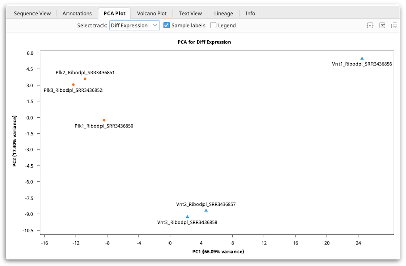
Principal Component Analysis for DESeq2 results

Principal component analysis (PCA) can be used to visualize variation between expression analysis samples. This method is especially useful for quality control, for example in identifying problems with your experimental design, mislabeled samples, or other problems.

When you perform a PCA, the normalized differences in expression patterns are used to compute a distance matrix. The X- and Y-axes in a PCA plot correspond to a mathematical transformation of these distances so that data can be displayed in two dimensions. This can make interpreting PCA plots challenging, as their meaning is fairly abstract from a biological perspective.

Creating a PCA Plot

A PCA plot will automatically be generated when you compare expression levels using DESeq2. This plot will be available to view in the PCA Plot viewer once you have saved the newly-generated differential expression sequence track to your document. If you have multiple differential expression tracks from running DESeq2 more than once, you will have the option to select which track you'd like to show in the PCA Plot viewer.

Interpreting PCA Plots

PCA is typically used primarily as a quality control or exploratory tool. In general, if your samples were produced under two experimental conditions (e.g. treated vs. untreated), the PCA plot should normally show that a) samples subjected to the same condition cluster together, and b) the clusters should be reasonably well-separated along the X-axis ("PC1": the first principal component).

An Example of Using PCA As An Exploratory Tool

The plot shown below shows data from a fictitious bacterial strain that could potentially be useful for bioremediation, cultured in the presence or absence of a halogenated industrial solvent ("Halogen"). The halogen is toxic to the two mutant strains, but not to the wild type. In this case, samples were compared according to the presence (blue) or absence (orange) of the halogen in the culture medium. The mutants contain a deletion in a transcriptional element thought to affect metabolism of the halogen, so the expected result is that expression levels in mutants would be similar to those of wild-type samples grown in the absence of the halogen.

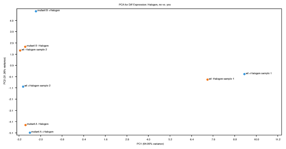
On inspection of the PCA plot above, two things are apparent:

1. The variance explained by the first principal component (X-axis) is not consistent with the expected result of this experiment, which is a strong indication that further investigation is required. Some possible explanations for this result are:

   • Perhaps two of the wild type samples were mislabeled and the sample labeled "wt -Halogen sample 1" was actually grown in the presence of the halogen and "wt +Halogen sample 2" without the halogen.

   • There could be some other explanation that should be investigated (e.g. contaminated medium, a malfunctioning incubator, etc.).

   • These samples might be outliers that you choose to discard.

2. The second principal component (Y-axis) explains quite a lot of variance, particularly the variance between the two mutant strains. While this result might be expected, it could also be interesting!

Volcano Plots

The Volcano Plot allows you to see the most highly differentially expressed loci. This is automatically generated when you compare expression levels using either Geneious or DESeq2. This plot will be available to view in the Volcano Plot viewer once you have saved the newly-generated differential expression sequence track to your document. If you have multiple differential expression tracks from running more than one analysis, you will have the option to select which track you'd like to show in the Volcano Plot viewer.

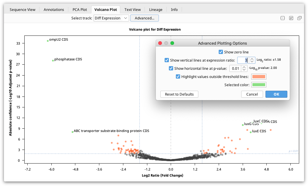
The Volcano Plot shows the fold change (log2 Ratio) plotted against the Absolute Confidence (-log10 adjusted p value). Each dot on the plot is one gene, and the "outliers" on this graph represent the most highly differentially expressed genes. Red asterisks are genes where the ratio is more than 10,000 or for which the p value is so tiny it is recorded as zero. As it's not possible to take the log of 0, the value is clipped so it is displayed at the higher ends but with an asterisk. To see the gene represented by each dot, mouse over the dot. Click the dot to select it and display the gene name on the graph. The dots on the Volcano plot are linked with both the annotations table and the annotations in the sequence viewer. Thus, if a locus is selected on the Volcano Plot, it will also be selected in the annotations table and the sequence viewer.

The Volcano Plot can be configured by clicking the Advanced button. Here you will find the following options:

• Show zero line: Shows a vertical line at log2 ratio = 0 (fold change = 1)

• Show vertical lines at expression ratio: Shows vertical lines at ± log2 ratio values.

• Show horizontal line at p value: Shows a horizontal line at the -log10 p value. "Significant" values will be above this line.

• Highlight values outside threshold lines: Highlights outliers defined by the specified p value and expression ratio thresholds. Loci with p values less than the threshold and log2 ratios outside the inter-quantile interval will be indicated by this color.

• Selected color: Dot color for selected loci.

Comparing Expression Levels Using the DESeq2 Method on Linux Systems

Before you can analyze RNA-Seq data using DESeq2 within Geneious on Linux, you will first need to install R and the DESeq2 package, following the instructions below. This is only necessary for Linux systems, as Geneious will automatically install R on Windows and MacOS systems the first time DESeq2 is run. Note that Geneious 2023.1.1 or newer is required for DESeq2 integration.

Once R has been installed, you will be able to run the DESeq2 method to Compare Expression Levels within Geneious like any other Geneious operation. You may need to specify the R executable location in the DESeq2 options, for example, if R is not installed on PATH.

Note that the installation instructions for R on Ubuntu, Centos or Red Hat Enterprise Linux require sudo or root access. If you do not have root access, you can install R from source in your home directory.

Installing R

Install R version 4.3 or greater. For more information, or more detailed instructions for select Linux distributions, refer to the R Project website.

R installation on Ubuntu:

1. On the terminal, enter the following commands to install R and its dependencies:

$ sudo apt-get update
$ sudo apt-get install libcurl4-openssl-dev libxml2-dev libssl-dev
$ sudo apt-get install r-base r-base-dev

1. You can now proceed with Installing DESeq2 (below)

R installation on Centos or Red Hat Enterprise Linux:

1. On the terminal, enter the following commands to install Rs dependencies:

$ sudo yum install curl
$ sudo yum install libcurl libcurl-devel
$ sudo yum install libxml2 libxml2-devel

1. Now install R with the following command:

$ sudo yum install R

1. You can now proceed with DESeq2 installation

R installation from source in your home directory

You should only install R from source in your home directory if you do not have root access.

1. Download the R source archive from the R project website

2. On the terminal, go to the directory where you downloaded the the source

3. Extract the archive:

$ tar -xvzf R-4.3.Y.tar.gz

(Replace 4.3.Y with the version you are installing)

1. Enter the source directory:

$ cd R-4.3.Y

1. Run the following commands to build and install R:

$ ./configure --prefix=$HOME/R
$ ./configure --prefix=$HOME/R

Note that if the first command fails because of missing libraries, it may still be possible to install these dependencies without root access.

This will install R in your home directory under $HOME/R/bin.

You can add this directory to your PATH variable or run R from the terminal with the command ~/R/bin/R.

You can now proceed with DESeq2 installation.

Installing DESeq2

Once you have installed R, you must install Bioconductor, then use Bioconductor to install DESeq2.

From the terminal, launch R normally using the command: R

1. Install Bioconductor:

if (!require("BiocManager", quietly = TRUE))
    install.packages("BiocManager")

1. Install DESeq2:

BiocManager::install("DESeq2")

Note that you will be asked to install any dependent packages that are not already installed. This step can take some time: wait for it to finish before proceeding

1. Quit R by entering CTRL-D. You will be asked whether you'd like to save your workspace image; you may answer 'n' (answer 'y' if you'd like to use R from the terminal in the future and wish to save the history of the commands you used).