Assembly and Mapping
Assembly is normally used to align and merge overlapping fragments of a DNA sequence (typically produced from Sanger or next-generation sequencing (NGS) sequence platforms) to reconstruct the original sequence. The assembly essentially appears as a multiple sequence alignment of reads (called the contig document) and the consensus sequence of the contig can be used for the reconstruction of the original sequence. Where positional information such as paired-end and mate-pair data is available, contigs can be joined into longer sequences called scaffolds.
Sequence assembly can refer either to de novo assembly or map to reference. De novo assembly focuses on the reconstruction of the original sequence by aligning and merging shorter reads, while map to reference consists of mapping reads to a reference sequence. The first approach is usually applied to genomes that have not been characterised yet, while the second one usually focuses on identifying differences from a well-characterised reference sequence.
Supported sequencing platforms
The Geneious assembler can handle data from Sanger and high-throughput (NGS) sequence platforms. Because different sequencing platforms have different error profiles and rates, they may require different assembly parameters. To ensure the optimal parameters are used for your dataset you can set the sequencing platform under Sequence → Set Read Technology. This can also be set during the file import process if you are importing fastq files.
The Geneious assembler works well with Sanger, Illumina, Ion Torrent, 454, and PacBio CCS data. PacBio CLR and Oxford Nanopore data are more problematic for Geneious due to the very high error rates. Depending on the data quality, you may be able to use these with map to reference, but are unlikely to be able to successfully de novo assemble them. We recommend using the plugins for Flye or Minimap2 for assembly and mapping of Oxford Nanopore and PacBio data, rather than using the Geneious assembler.
When de novo assembling only Illumina sequencing data, turning off 'Allow gaps' (in the advanced options) can sometimes improve performance and results. If any of the input sequences are set as PacBio or Oxford Nanopore, Geneious will automatically use a maximum gap size of 2 to 3 times the specified value.
Both the Geneious de novo assembler and mapper will also work with arbitrarily long reads. For example, you can use high quality contig consensus sequences as input to either of these.
Read processing
Setting paired reads
To assemble paired read (or mate pair) data, prior to assembly you first need to tell Geneious the reads are paired. The assembler will then automatically used the paired data unless you turn off the advanced option to Use paired distances.
Paired reads can be set up either during the fastq import process, or by selecting the documents(s) containing the paired reads and going to Set Paired Reads from the Sequence menu.
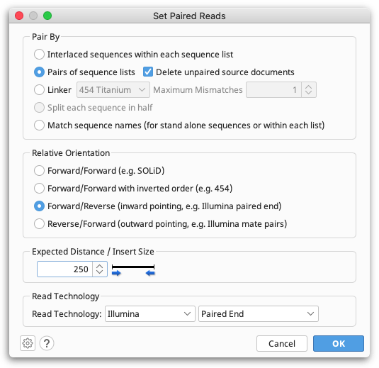
Depending on your data source, reads could be in parallel sets of sequences, or interlaced, so you need to select the appropriate format. Geneious will guess and select the appropriate option based on the data you have selected, so most of the time you can just use the default value for this. However, you must make sure you select the correct Relative Orientation for your data. Different sequencing technologies orientate their paired reads differently. All paired read data will have a known expected distance between each pair. It is important you set this to the correct value to achieve good results when assembling. If you don't know what the relative orientation or expected distance is between the reads you should ask your sequencing data provider.
When you click 'OK', if you chose to pair by parallel lists of sequences a new document containing the paired reads will be created. If you do this during the fastq import process, Geneious will only import the paired read file and not the original unpaired files. If you chose to pair an interlaced list of sequences (or modify settings for some already paired data), the existing list of sequences will be modified to mark it as paired.
If you choose to split reads based on the presence of a linker sequence (e.g. for 454 data) the original sequences will be unmodified and the split reads will be created in a new document. The default behaviour is to ignore sequences shorter than 4 bp either side of the linker, but this can be customized from the Edit Linkers option in the paired reads options.
Polonator sequencing machine reads can be split using the Split each read in half option.
Trim Ends
Trimming low quality ends of sequences is normally performed before assembling a contig. This is because the noise introduced by low quality regions and vector contamination can produce incorrect assemblies. Geneious contains built-in read trimmers under either Trim Ends or Trim Using BBDuk option. BBDuk is a powerful NGS trimmer with some additional options not present in the Geneious trimmer. Geneious Prime 2023 onwards BBDuk comes as a bundled plugin with Geneious application and does not require a separate installation.
To trim and filter using the Geneious tool, select the sequences you wish to trim and choose Annotate and Predict → Trim Ends. This option allows you to trim vectors, primers and poor quality bases and filter out reads by length. It can also be performed at the assembly step, by checking the trim sequences option in the assembly set-up.
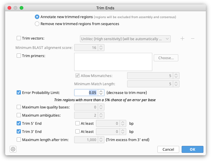
Trim Ends can soft or hard trim your sequences. If you wish to soft trim, choose to Annotate new trimmed regions in the Trim Ends set up. The trimmed sequence will then remain visible but will be annotated with "Trimmed" annotations. Sequence annotated with a trimmed annotation is ignored by the assembler when constructing a contig and will not be included in the consensus sequence calculation. So although the trimmed regions are visible, they do not affect the results of the assembly at all. Soft trims can be adjusted as needed, or deleted completely. Dragging the ends of the trim annotation will make the newly untrimmed sequence visible and part of the consensus.
If you wish to remove the trimmed sequence completely (hard trim), choose Remove new trimmed regions from sequences.
If you choose to trim your sequences at the assembly step, the sequences are trimmed and assembled in one operation and you will not be able to view the trimming before assembly is performed. However, the trimmed regions will still be available and adjustable after assembly is complete. If you choose to trim your sequences prior to assembly, select Use Existing Trim Regions when you set up the assembly.
Trimmed annotations can also be created manually using the annotation editing in the sequence viewer. If you create annotations of type Trimmed and save them, then Geneious will treat them the same as ones generated automatically and they will be ignored during assembly. Trimmed annotations can also be modified in this way before or after assembly.
Trim Ends options
-
Annotate new trimmed regions: Calculate new trimmed regions and annotate them - the trimmed regions will be ignored when performing assembly and calculating the consensus sequence.
-
Remove new trimmed regions from sequences: Calculate new trimmed regions and remove them from the sequence(s) completely. This can be undone in the Sequence View before the sequences are saved.
-
Remove existing trimmed regions from sequences: This is only available when there are already trimmed regions on some of the sequences. This will remove the existing trimmed regions from the sequences permanently; no new trimmed regions are calculated.
-
Trim vectors: Screens the sequences against UniVec or your own custom BLAST database to locate any vector contamination and trim it. This uses an implementation similar to NCBI's VecScreen to detect contamination (http://www.ncbi.nlm.nih.gov/projects/VecScreen/). Multiple databases can be selected to trim from by clicking the + sign.
-
Trim primers: Screens the sequences against primers in your local database.
-
Error Probability Limit: Available for chromatogram documents which have quality (confidence) values. The ends are trimmed using the modified-Mott algorithm (see below) based on these quality values (Richard Mott personal communication).
-
Maximum low quality bases: Specifies the maximum number of low quality bases that can be in the untrimmed region. Low Quality is normally defined as confidence of 20 or less. This can be adjusted on the Sequencing and Assembly tab of Preferences.
-
Maximum Ambiguities: Finds the longest region in the sequence with no more N's than the maximum ambiguous bases value and trims what is not in this region. This should be used when sequences have no quality information attached.
-
Trim 5' End and Trim 3' End: These can be set to specify trimming of only the 3' or 5' end of the sequence. A minimum amount that must be trimmed from each end can also be specified.
-
Minimum length after trim: If the length of the sequence after trimming is less than the number specified here then the sequence is discarded. This option is useful for filtering out sequences that are too short to be useful after trimming.
-
Maximum length after trim: If the untrimmed region is longer than the specified limit then the remainder will be trimmed from the 3' end of the sequence until it is this length.
The Modified Mott algorithm
The modified-Mott algorithm for trimming ends based on quality operates as follows:
For each base, it subtracts the base error probability from an error probability cutoff value (default 0.05) to form the base score. The base error probability is calculated from the quality score (Q), such that P(error)=10(Q/-10). This means that low quality bases have high error probabilities and thus may have a negative base score.
E.g. For Q10, P(error)= 0.1, For Q30, P(error)=0.001
So with an error probability cutoff of 0.05, a base with Q10 has a base score of 0.05-0.1= -0.05, and a base with Q30 would have a base score of 0.05-0.001=0.049.
The trimming algorithm then calculates the running sum of the base score across the sequence. If the sum drops below zero it is set to zero. The part of the sequence not trimmed is the region between the first positive value of the running sum and the highest value of the running sum (i.e. the highest scoring segment of the sequence). Everything before and after this region is trimmed.
Operations that respect soft trims
The following operations will exclude sequence that has been soft trimmed:
-
De novo assembly*
-
Map to Reference*
-
Multiple and pairwise alignment (all algorithms)
-
Find Variants/SNPs
-
Remove Chimeric reads
-
Calculation of consensus sequence
-
Calculation of sequence identity (displayed in statistics tab and identity graph)
-
Calculation of coverage (displayed in statistics tab and coverage graph)
-
Calculation of confidence mean / quality score outputs. This includes the outputs shown in the statistics tab, the calculation of HQ%, MQ% and LQ%, and corresponding sequence bins based on those figures.
-
Document fields: Ambiguities (chromatograms), Post-Trim (length of sequence after trimming)
*Only the Geneious assembler supports the use of trimmed annotations. Sequences should be hard trimmed if using other assembly algorithms, such as SPAdes, Tadpole, Bowtie etc.
Operations that do not respect soft trims
The following operations will include sequence that has been soft trimmed:
-
Calculation of nucleotide/amino acid frequencies and molecular weights
-
Calculation of sequence lengths (including lengths graph)
-
Dotplot
-
BBTools operations, including "Trim with BBDuk", "Merge Paired Reads", "Remove Duplicate Reads", and "Error correct and normalize"
-
Mask Alignments
-
Export formats fasta/fastq, Mega, Nexus, Phylip, CSV/TSV
Export formats SAM/BAM, Genbank, GFF, and ACE incorporate the trim information in the export.
Merging paired reads
If paired reads were sequenced with an insert size shorter than twice the read length then pairs may overlap with each other, in which case it can be useful merge to each pair into a single longer read. This is usually performed for Amplicon sequencing. After setting up paired reads (see Setting Paired Reads) use Merge Paired Reads... from the Sequence menu to merge them.
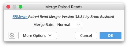
This function uses BBMerge from the BBtools suite. For a detailed explanation of any BBMerge setting, hover the mouse over the setting, or click the help (question mark) button next to the custom options under More Options.
Alternatively, an experimental plugin for merging paired reads using FLASH is available from the Geneious website plugins page.
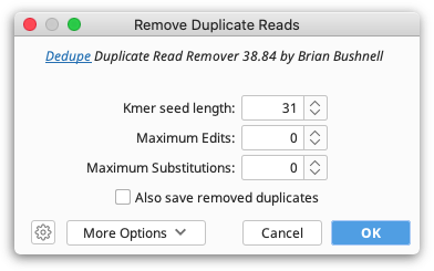
Removing duplicate reads
To remove duplicate reads from NGS datasets, use Remove Duplicate Reads... under the Sequence menu. This function runs Dedupe, and will remove duplicate sequences that are either exact matches, subsequences, or sequences within some percent identity. It can also find overlapping sequences and group them into clusters. For a detailed explanation of any Dedupe setting, hover the mouse over the setting, or click the help (question mark) button next to the custom options under More Options.
Removing chimeric reads
To remove chimeric reads from NGS datasets, select the sequence list containing your reads and go to Sequence → Remove Chimeric Reads. This runs UCHIME by Robert Edgar and is typically used to remove PCR chimeras from amplicon sequencing (e.g. 16S, ITS). The public domain version of UCHIME is provided with Geneious. If you would prefer to detect chimeric sequences using USEARCH, which contains a much faster version of the UCHIME algorithm, you can optionally specify a USEARCH executable instead.
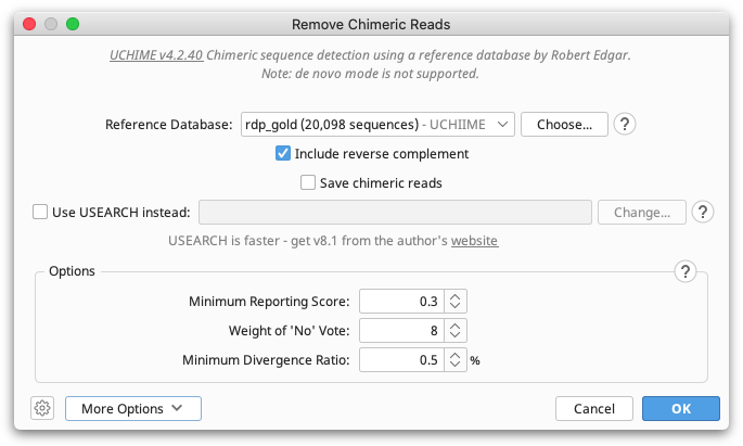
Geneious supports reference mode only, and you must supply the reference database yourself. This may be either a nucleotide sequence list or a nucleotide alignment in your Geneious database. Information about common reference databases for 16S rRNA or fungal ITS sequences is available, along with links to download locations, on the Geneious knowledge base. When you have imported your preferred database into Geneious, choose this document as the Reference Database.
If your query sequences are paired, you may need to run Merge paired reads before chimera detection. When a query sequence list with reads set as paired is selected, Geneious will always consider both members of a pair to be chimeric if either is identified as such. Note that UCHIME does not recognize paired reads, therefore by default Geneious will concatenate paired reads and submit each pair to UCHIME as a single sequence. This should generally be appropriate for reads that are separated by small gaps. To override this setting, you can check Run paired reads separately under More Options.
The following options are available for configuration within Geneious should you wish to optimize the settings for your data. The default settings in Geneious are consistent with the UCHIME defaults.
-
Include reverse complement: UCHIME looks only at the sequences provided in the reference database. You should check the Include reverse complement box if you would like Geneious to submit both the reference database sequences and the reverse complement of each to UCHIME.
-
Save chimeric reads: This will save the chimeras that are removed as a separate list. Ordinarily only those reads identified as non-chimeric would be saved, so choose this option if you want the chimeric sequences for any subsequent steps or analysis.
-
Use USEARCH executable: The USEARCH implementation of UCHIME is also supported. To use it you must first navigate to the USEARCH download page, register for a licence, and then download USEARCH. Currently Geneious supports USEARCH v8.x. Once downloaded check the Use USEARCH executable instead box and specify the location of the file you downloaded.
-
Minimum score to report chimera: The minimum score at which a sequence is considered a chimera. Values from 0.1 to 5.0 are considered reasonable. Lower values increase sensitivity but may result in more false positives. This may need to be changed as the weight of a no vote and minimum divergence ratios are changed.
-
Weight of a no vote: The UCHIME algorithm uses a voting system when determining the score of each read. This option specifies the weight of each no vote. Increasing this option tends to result in lower scores. Decreasing to around 3 or 4 may give better performance on denoised data.
-
Minimum divergence ratio: This option is used to allow some flexibility in what is considered chimeric, by allowing you to specify the allowed percent divergence between the query and the closest reference database sequence. The default (0.5%) allows chimeras that are up to 99.5% similar to a reference sequence. This is useful when you are not concerned with chimeras that are similar to the parent sequences.
-
Run paired reads separately: Tells Geneious not to concatenate paired reads prior to running UCHIME. This is useful when there is a long insert between members of a pair and running them as a pair may lead to increased false negatives. Note that Geneious will consider both members of a pair as chimeric if either is classified as such by UCHIME, irrespective of whether this option is selected.
-
Number of chunks: This option specifies the number of non-overlapping segments (chunks) that the query sequence is divided into. Each chunk is used to search the reference database.
-
Sequence length: By default UCHIME is designed to operate on sequences between 10 bp and 10,000 bp. This can be altered by changing the Minimum sequence length and Maximum sequence length under More Options. Altering the valid sequence lengths may be necessary when reads are paired and concatenated because the new read length is the sum of both pairs. Similarly, the minimum sequence length needs to be considered when trimmed reads are present, as Geneious will perform a hard trim before running UCHIME.
-
Custom UCHIME options: Geneious supports sending additional options to UCHIME. This is done by entering the desired options into the Custom UCHIME options field found under More Options. You can use any of the options that UCHIME would normally support as long as they are not input/output options and do not overlap with the options provided by Geneious. It is up to you to ensure these are valid. When using a custom USEARCH executable, refer the appropriate user guide for available command line options. The following options are provided by Geneious: UCHIME:
–input,–db,–uchimeout,–uchimealns,–minh,–xn,–mindiv,–chunks,–minlen,–maxlenUSEARCH:–uchime_ref,–strand,–minseqlength,–maxseqlength,–uchimeout,–db,–uchimealns,–minh,–xn,–mindiv,–chunks
Error correction and normalization of reads
Prior to de novo assembly, it can sometimes be useful to error correct the data or to normalize coverage by discarding reads in regions of high coverage. This functionality is available using Error Correct & Normalize Reads... from the Sequence menu.
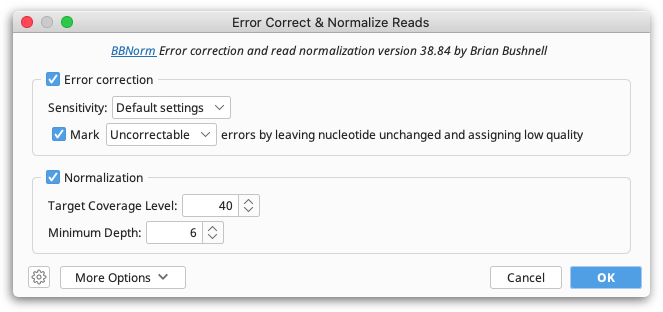
This function uses BBNorm from the BBtools suite. For a detailed explanation of any BBNorm setting, hover the mouse over the setting, or click the help (question mark) button next to the custom options under More Options. For more information, see the BBNorm page on SeqAnswers.
Splitting multiplex/barcode data
Multiplex or barcode data can be separated using Separate Reads by Barcode from the Sequence menu. This function copies all sequences matching a given barcode to a correspondingly named sequence list document.
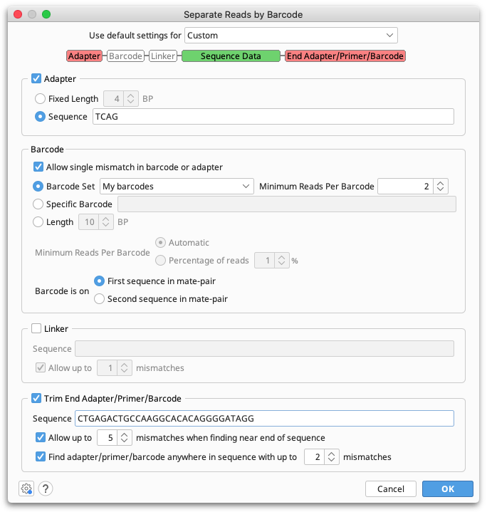
Default settings are provided for 454 standard and Titanium MID barcodes (with or without Adaptor B trimming), and Rapid MID barcodes. These settings recognise standard MID sequences provided by 454 and use their names when appropriate.
To enter a custom barcode set, select Custom settings, then under Barcode set choose Edit barcode sets. Then click Add to add your list of barcodes. To specify fixed sequences either side of the barcode, enter these in the Adaptor and Linker sections.
If you only want to extract sequences with a single, specific barcode sequence (e.g. a primer), check Specific barcode and enter the sequence. Alternatively if you do not know your barcode sequences, you can just enter the length of your barcodes and Geneious will automatically identify what the barcodes are.
Separate reads by barcodes only sorts by barcodes at the 5' end of the sequence, but primers, adapters or barcodes on the 3' end of the sequence can be trimmed off by checking Trim End Adaptor/Primer/Barcode. Either enter a specific sequence to trim, or add your 3' barcode to your custom barcode set and use the text [END_BARCODE] in the sequence box. Primer trimming can also be performed after separating by barcodes using Trim Ends.
For further information on splitting barcode data, hover the mouse over any of the settings in the Separate Reads by Barcode options window.
De novo assembly
This can be used to assemble a small number of Sanger sequencing reads (i.e. forward and reverse reads of the same sequence), or millions of reads generated by NGS platforms such as Illumina, 454, Ion Torrent and PacBio CCS. To assemble a contig firstly select all of the sequences and/or contigs you wish to assemble in the document table then click Align/Assemble in the toolbar and choose De Novo Assemble. The basic options for de novo assembly will then be displayed.
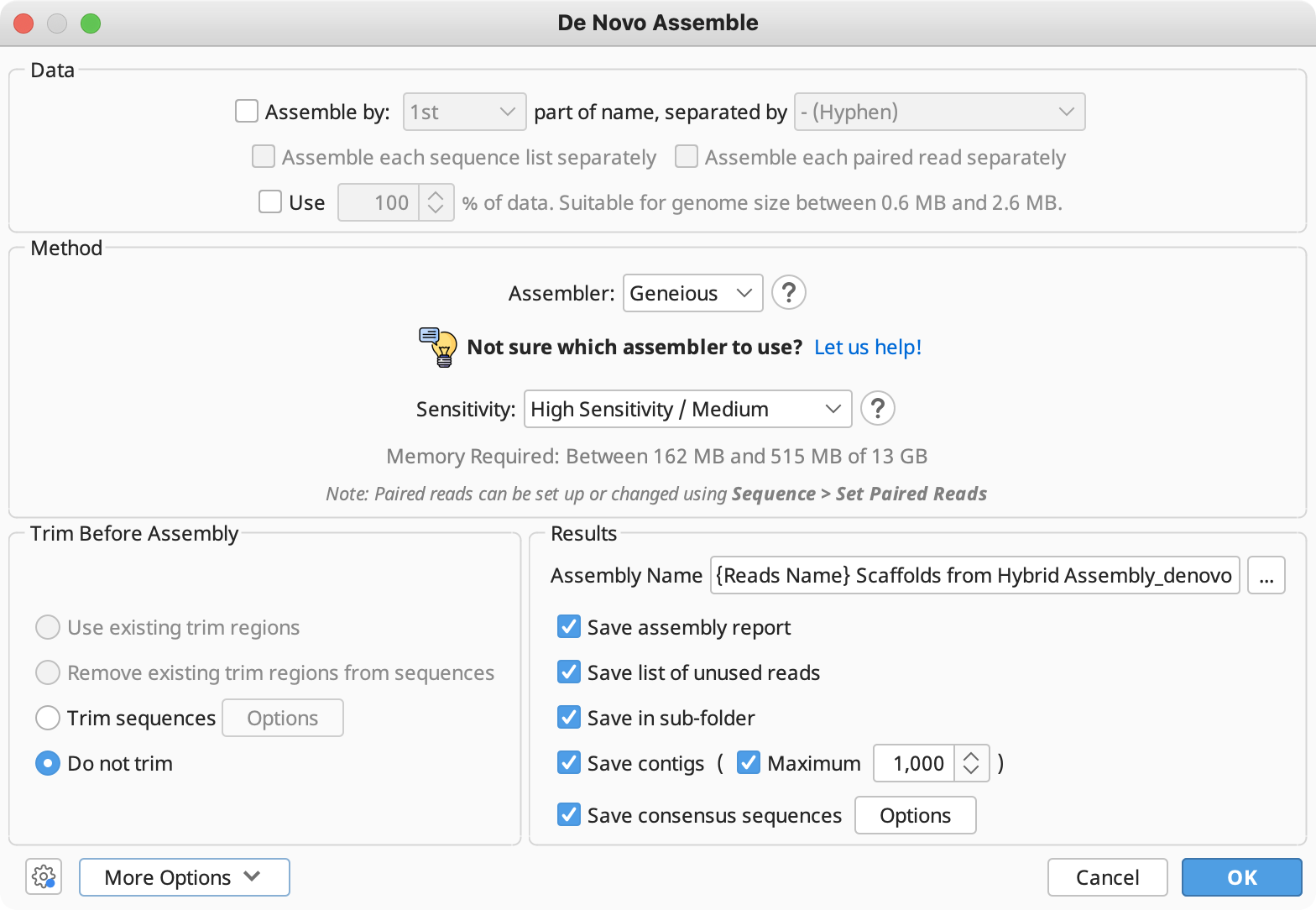
The options available here are as follows:
-
Assemble by (aka Assemble by Name): If you have selected several groups of fragments which are to be assembled separately, you can specify a delimiter and an index at which the identifier can be found in all of the names. Sequences are grouped according to the identifier and each group is assembled separately. If a reference sequence is specified, it is used for all groups. eg. For the names A03.1.ab1, A03.2.ab1, B05.1.ab1, B05.2.ab1 etc where "A03" and "B05" are the identifiers you would choose "Assemble by 1st part of name, separated by . (full stop)"
-
Use % of data: This option is will show with large datasets and enables you to assemble a subset of your data, rather than the full dataset. For example, if you enter 20% here, then the first 20% of reads in a sequence list will be assembled and the rest will be ignored. This is useful in situations where the full dataset is too large for the size of genome being assembled.
-
Assembly method: In this section you can choose from the built-in Geneious assembler, or SPAdes, Velvet, MIRA and Flye assemblers if you have these plugins installed. Click the question mark button next to the method to see a list of the advantages and disadvantages of each assembler. Click "Let us help" to start the assembly advisor. By answering some quick questions about your data, Geneious' assembly advisor can guide you to the recommended assembly method(s).
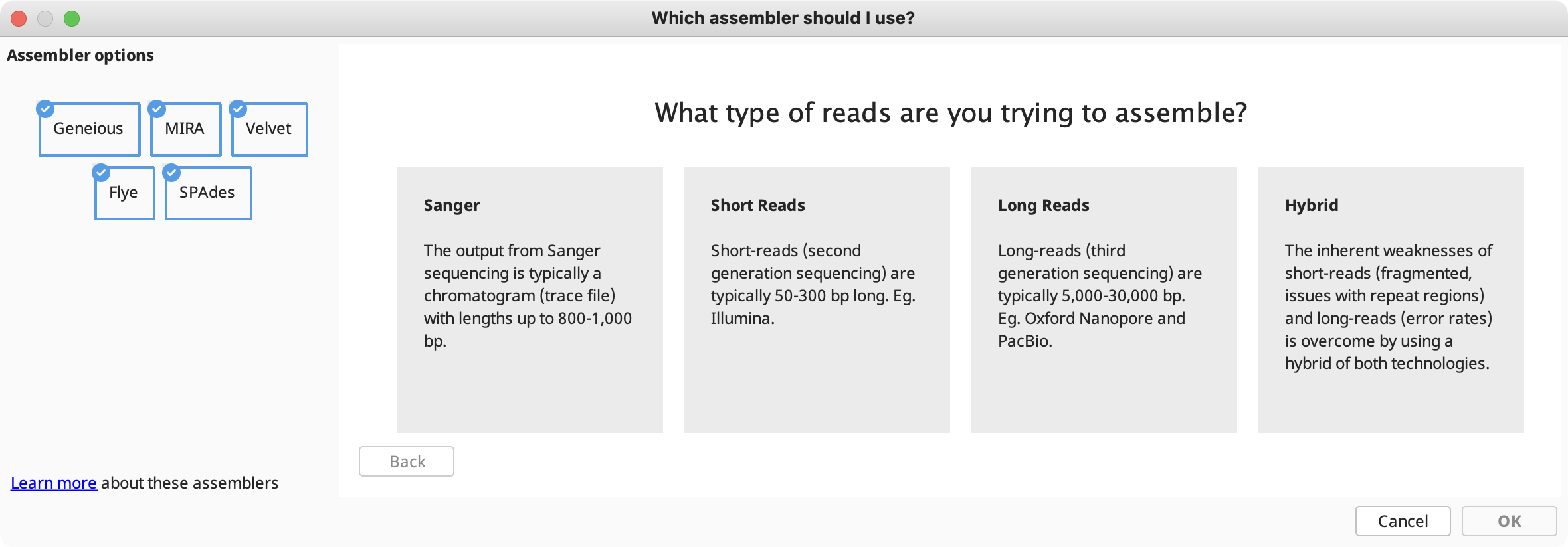
The assembly advisor will guide you through the decision tree below to suggest the most appropriate assembly algorithm. Support for each decision can be found in the denovo assembly advisor decision tree validation table.
- Sensitivity (Geneious assembler only): specifies a trade off between the time it takes to assemble and the accuracy of the assembly. Higher sensitivity is likely to result in more reads being assembled.
- Trim Sequences: Select how to trim the ends of the sequences being assembled. See Trim Ends.
- Results: Allow you to choose an assembly name and what to return in your results. By default, only the assembled contigs are saved, but you can also choose to return an assembly report, lists of used or unused reads and the consensus sequences. The assembly report summarises the assembly statistics and lists which fragments were successfully assembled and which contig they went in to along with a list of unassembled fragments. If Save in Subfolder is selected all the results of the assembly will be saved to a new subfolder inside the one containing the fragments. This folder will always only contain the assembly results from the one most recent assembly - it creates a new folder each time it is run.
- More Options: Under the advanced options you can change the parameters used by Geneious when aligning fragments together. These are fully documented if you hover the mouse over them in Geneious. To edit these settings, you must first choose Custom Sensitivity in the assembly method panel. For sequences which are lower quality or contain many errors, or are expected to be divergent from one another, you may need to decrease the minimum overlap identity and maximum mismatches per read, and increase the maximum gaps allowed per read.
Choose the options you require and click 'OK' to begin assembling the contig. Once complete, one or more contigs may be generated. If you got more contigs than you expect to get for the selected sequences then you should try adjusting the options for assembly. It is also possible that no contigs will be generated if no two of the selected sequences meet the overlap requirements.
Note: The orientation of fragments will be determined automatically, and they will be reverse complemented where necessary.
If you already have a contig and you want to add a sequence to it or join it to another contig then just select the contig and the contig/sequence and click de novo assembly as normal.
Scaffolding
Scaffolds are contigs which are linked together, with the missing regions between them filled by Ns. The size of the missing region is based on paired read distances. The Geneious assembler will produce scaffolds if this option is turned on under More options. If this setting is disabled it is because your data does not have paired reads or you haven't marked the data as paired using Set Paired Reads from the Sequence menu.
Unlike some assemblers where scaffolding is performed after contig formation, Geneious scaffolding is integrated into the contig assembly process. When there is strong support for scaffolding, it may take precedence over potentially conflicting standard contig formation. For this reason, Geneious can't be configured to produce both scaffolds and non-scaffolds from a single run.
De novo assembly of circular genomes
The Geneious de novo assembler can produce a circular contig if you are working with a circular genome. To enable this option, click the More Options button and check Circularize contigs of [x] or more sequences, if ends match. Circularization requires that the ends of the contig match, and that the contig contains at least the number of specified sequences.
A circular contig will contain reads at either end marked with arrows, which denotes that these reads span the origin and link back around to the other end of the assembly. The consensus sequence produced from this contig will also be circular. The Topology column in the Document table lists whether a given contig is circular or linear.
The de novo assembly algorithm
The sequence assembler in Geneious is flexible enough to handle read errors consisting of either incorrect bases or short indels. It can handle reads of any length, including paired-reads and mixtures of reads from different sequencing machines (hybrid assemblies).
De novo assemblers are generally either overlap or k-mer (De Bruijn graph) based. The Geneious de novo assembler is an overlap assembler which uses a greedy algorithm similar to that used in multiple sequence alignment.
-
For each sequence a blast-like algorithm is used to find the closest matching sequence among all other sequences.
-
The highest scoring sequence and its closest matching sequence are merged together into a contig (reverse complementing if necessary). This process is repeated, appending sequences to contigs and joining contigs where necessary.
-
For paired read de novo assembly, 2 sequences with similar expected mate distances are given a higher matching score if their mates also score well against each other. Similarly a sequence and its mate will be given a higher score if they both align at approximately their expected distance apart to an already formed contig. The effect of this heuristic is that paired read de novo assembly starts out by finding 2 sets of paired reads and forming 2 contigs. Each of these 2 contigs will contain 1 sequence from each pair and the 2 contigs are expected to be separated by the expected mate distance. Assembly proceeds from there either adding new paired reads to the contigs or forming new pairs of contigs which eventually merge together. Due to the nature of this algorithm, paired read de novo assembly in Geneious only works well if you have high coverage of paired reads - a hybrid assembly of mostly unpaired data with a few paired reads will not make good use of the paired read data, but this is expected to improve in future versions.
-
Each contig generated by a gapped de novo assembly has some minor fine tuning performed on it both during assembly and upon completion. For each gapped position in a sequence, a base adjacent to the gap is shuffled along into the gap if it is the same base as the most common base in other sequences in the contig at that position. After doing this if any column now consists entirely of gaps that column is removed from the contig
-
Other heuristics are applied throughout the assembly to improve the results such as identifying repeat regions
-
Both the Geneious de novo and reference assemblers use a deterministic method (even when spreading the work cross multiple CPUs) such that if you rerun the assembler using the same settings and same input data it will always produce the same results.
Map to reference
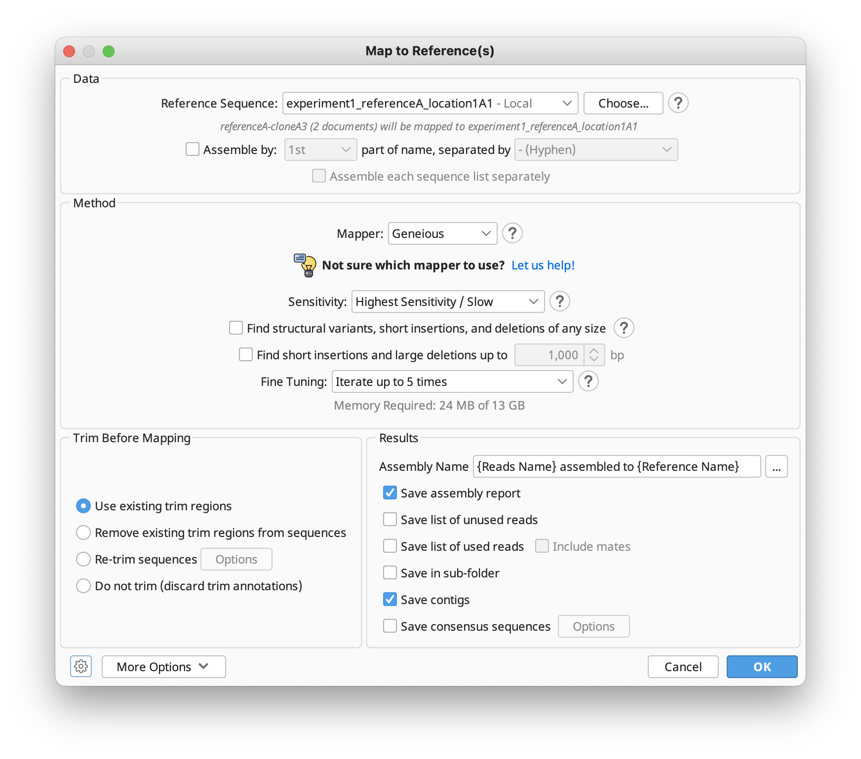
Map to Reference is used when you wish to assemble sequences to a known sequence, for example to locate differences or SNPs. To perform assembly to a reference sequence select your sequences and click Align/Assemble and choose Map to Reference. Choose the name of the sequence you wish to use as the reference in the Reference Sequence chooser and click OK. One contig will be produced per reference and this will display the reference sequence at the top of the alignment view with all other sequences below it.
The options available in the Map to Reference setup dialog are similar to those for De Novo Assembly, with a few differences detailed in the subsequent sections. In the Methods panel, you can choose between the standard Geneious assembler, Geneious for RNAseq, STAR (Geneious Prime 2023+) or the BBMap, Bowtie, Minimap2 (Geneious Prime 2020+) mappers if you have these plugins installed.
If you're not sure which mapper to use, Click "Let us help" to start the assembly advisor. By answering some quick questions about your data, Geneious' assembly advisor can guide you to the recommended map-to-reference assembly method(s).
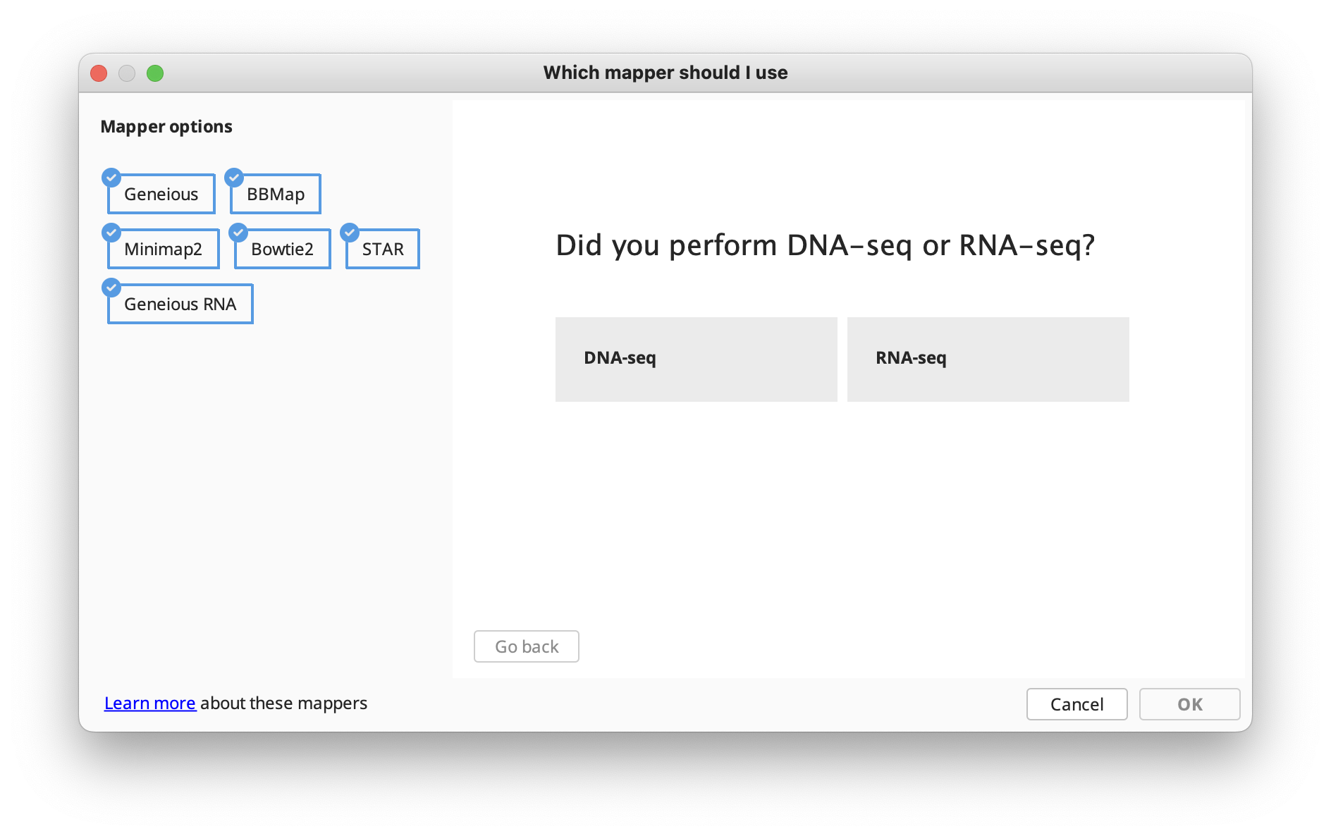
The assembly advisor will guide you through the decision tree below to suggest the most appropriate assembly algorithm. Support for each decision can be found in the Map-to-Reference assembly advisor decision tree validation table.
Choosing reference sequences
In version 8.1 and above, it is not necessary to select the reference sequence prior to choosing Map to Reference. Instead, the reference sequence can be chosen from within the Map to Reference setup options by clicking Choose.... This brings up a document chooser from which you can select single or multiple reference sequences from any folder in your database.
Multiple reference sequences may be selected either by choosing a sequence list containing your reference sequences, or by selecting multiple sequence documents using the Choose... button. Single reference sequences may be pre-selected prior to choosing the Map to reference... option, however when using the Choose... button, only those documents selected within the Choose... dialog will be used as reference sequences (all other sequences will be mapped).
If multiple reference sequences are selected, each read will be mapped to the sequence with the best match only, and will produce one contig per reference. Batch assemblies where each read gets mapped to each reference sequence can be done by using Workflows → Map reads to each reference sequence.
Fine tuning
When aligning to reference the sequences are not aligned to each other, each of them is instead aligned to the reference sequence independently and the pairwise alignments are combined into a contig. However, an iterative fine tuning step can be enabled, which makes reads that overlap from the initial assembly stage align better to each other. Fine tuning causes reads to align better to each other around indels which improves the accuracy of consensus and variant calling. For more information, click the help (question mark) button next to the fine tuning options in the Map to Reference setup dialog.
If you just wish to use a reference sequence to help construction of the contig where the reads extend beyond the length of the reference then you have two options. With iterative fine tuning, reads can extend a bit further past the ends of the reference sequence on each iteration so make sure you set the number of iterations high enough. Or you could select all sequences including the reference and use the De Novo assembler.
Deletion, insertion and structural variant discovery (DNA mapping)
Geneious can discover structural rearrangements, short insertions, and arbitrarily large deletions from paired or unpaired reads by analyzing how fragments of each read align to different regions of the reference sequence(s). To enable this option, check Find structural variants, short insertions and deletions of any size. If you only want to find deletions up to a specified size, check Find short insertions and large deletions up to...
For this operation, Geneious makes two passes during mapping. On the first pass each read mapped will generate candidate junctions (sites for structural variants) based on where fragments of the read align to different regions of the reference sequence(s). The more reads that support a candidate junction, the more likely it will be used during the second pass. The second pass involves mapping reads using the discovered junctions.
Insertions, where the ends of a read map to nearby locations but the center of the read doesn't map, are also detected. Since discovered insertions must be less than the read length, only short insertions are generally discovered. Only the most common insertion at a each position will be annotated and have reads correctly aligned with it.
By default, at least 2 reads must support the discovery of a junction in order for it to be used during the next pass. This threshold can be adjusted under More Options by changing the Minimum support for structural variant discovery setting. Insertion discovery can also be disabled here by unchecking Include insertions in structural variants.
Junctions used during the second mapping pass are annotated on the reference sequence under a track named after the reads. Annotations are only created for variants which are at least 3 bp in size. Each junction annotation has the following properties:
-
Junction Type: This will be Insertion for short insertions and Deletion for deletions up to 1000 bp. For longer deletions or structural variants, this will be Rearrangement, with (inversion) potentially appended.
-
Intervals: Junctions of type Insertion are shown as one single interval annotation covering the gapped region in the contig, or when viewed on the unaligned reference sequence, positioned between the nucleotides on either side of the insertion. Junctions of type Deletion and Rearrangement are each represented with two 1-bp annotation intervals positioned on the last nucleotide before the read jumps and continues elsewhere. For Deletions, this is a single annotation with two linked intervals. For Rearrangements, the junction site is split into two separate annotations, each with a jagged edge on one side of the interval to indicate the side which jumps elsewhere.
-
Deletion Size: This is present when Junction Type is Deletion.
-
Rearrangement Distance: This is present when Junction Type is Rearrangement to indicate the distance between the two junction sites.
-
Insertion Size: This is present when Junction Type is Insertion to indicate the number of nucleotides in the insertion.
-
Insertion: This is present when Junction Type is Insertion to indicate the nucleotides inserted.
-
Reads supporting discovery: Indicates the number of reads that supported discovery of this junction during the first pass. This may be lower than the advanced minimum support setting in cases where other reads supported discovery of a slightly offset version of this junction, which allows this junction to be retained on the next pass.
-
Reads using: Indicates the number of reads that used this junction as part of their mapping during the second pass.
-
Junction Source & Junction Destination: Clickable links to the junction positions in the reference sequence. When the destination is a different reference sequence, this is prefixed with the sequence name followed by a colon.
-
Color: Annotations are colored from blue to green based on increasing values of Reads supporting discovery. At 5 and above the color is fully green.
Reads spanning junctions may be represented in one of three possible ways:
-
For insertions, the insertion is represented as a gap in the reference sequence.
-
For deletions under 1,000 bp, the deletion is represented as a gap in the read. This gap contributes towards calling a gap in the consensus sequence.
-
For longer deletions or for structural variants, two copies of the read appear in the contig where the fragment of the read extending past the junction is marked as trimmed. Trimmed regions do not contribute to consensus sequence calling. These trim regions will only be visible when in editing mode. When not in editing mode, the trimmed regions will appear as 3 gaps fading to light grey. Clicking on these fading gaps will jump to the read at the other end of the junction. Faded gaps depend on the presence of the junction track created at the time of mapping. If these annotations are deleted, the faded gaps will appear as trimmed regions instead.
RNAseq mapping
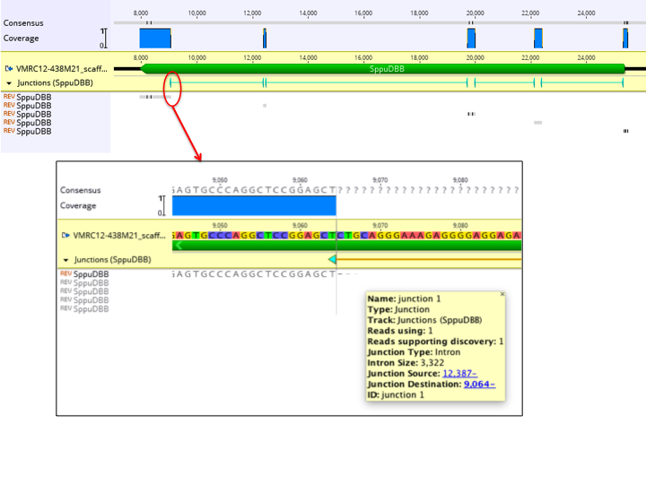
To map RNA sequence reads to a genome with introns, choose Geneious RNA as the Mapper in the Map to Reference setup dialog. This function can map reads that span existing annotated introns, or discover insertions, novel introns and fusion genes.
This function works in the same way as deletion and structural variant discovery for DNA mapping, by analyzing how fragments of each read align to different regions of the reference sequence(s), and creating a junction annotation at the point where the read is split. By default, at least 2 reads must support the discovery of a junction in order for it to be annotated. This threshold can be adjusted under More Options by changing the Minimum support for intron/fusion gene discovery setting.
If Span annotated mRNA introns is checked, junctions will be created from existing annotations on the reference sequence. Reads are still allowed to map anywhere, but will be allowed to freely span these junctions if that produces the best mapping.
To only find introns up to a certain size, check Find novel introns up to...; to find introns of any size, insertions, or structural rearrangements that may indicate a fusion gene, use Find fusion genes and novel introns.
As for deletion and structural variant discovery, junctions are annotated on the reference sequence under a track named after the reads. Each junction has the following properties:
-
Junction Type: This will be Insertion for short insertions. For introns under 2,000,000 bp, this will be Intron. For longer introns or structural variants, this will be Fusion, with (inversion) potentially appended.
-
Intervals: Junctions of type Insertion are shown as one single interval annotation covering the gapped region in the contig, or when viewed on the unaligned reference sequence, positioned between the nucleotides on either side of the insertion. Junctions of type Intron and Fusion are each represented with two 1-bp annotation intervals positioned on the last nucleotide before the read jumps and continues elsewhere. For Introns, this is a single annotation with two linked intervals. Introns that have common start and finish nucleotides will be assigned an appropriate direction. For Fusions, the junction site is split into two separate annotations, each with a jagged edge on one side of the interval to indicate the side which jumps elsewhere.
-
Intron Size: This is present when Junction Type is Intron.
-
Fusion Distance: This is present when Junction Type is Fusion to indicate the distance between the two junction sites.
-
Insertion Size: This is present when Junction Type is Insertion to indicate the number of nucleotides in the insertion.
-
Insertion: This is present when Junction Type is Insertion to indicate the nucleotides inserted.
-
Reads supporting discovery: Indicates the number of reads that supported discovery of this junction during the first pass. This may be lower than the advanced minimum support setting in cases where other reads supported discovery of a slightly offset version of this junction, which allows this junction to be retained on the next pass.
-
Reads using: Indicates the number of reads that used this junction as part of their mapping during the second pass.
-
Junction Source & Junction Destination: Clickable links to the junction positions in the reference sequence. When the destination is a different reference sequence, this is prefixed with the sequence name followed by a colon.
-
Color: Annotations are colored from blue to green based on increasing values of Reads supporting discovery.
Reads spanning junctions may be represented in one of three possible ways.
-
For insertions, the insertion is represented as a gap in the reference sequence.
-
For introns under 15 bp, the deletion is represented as a gap in the read. This gap contributes towards calling a gap in the consensus sequence.
-
For longer introns or for fusion genes, two copies of the read appear in the contig where the fragment of the read extending past the junction is marked as trimmed. Trimmed regions do not contribute to consensus sequence calling. These trim regions will only be visible when in editing mode. When not in editing mode, the trimmed regions will appear as 3 gaps fading to light grey. Clicking on these fading gaps will jump to the read at the other end of the junction. Faded gaps depend on the presence of the junction track created at the time of mapping. If these annotations are deleted, the faded gaps will appear as trimmed regions instead.
The figure below shows an example of a single cDNA sequence mapped to a genomic sequence. In the zoomed out view above, the coverage graph and junction annotation track provides a quick view of where the cDNA maps to the genomic sequence. Five copies of the cDNA sequence appear in the contig, as it maps across 5 exons. The inset shows a zoomed in view of a junction, with the junction annotation properties shown.
The map to reference algorithm
The reference assembly algorithm used is a seed and expand style mapper followed by an optional fine tuning step to better align reads around indels to each other rather than the reference sequence. Various optimizations and heuristics are applied at each stage, but a general outline of the algorithm is
- First the reference sequence(s) is indexed to create a table making a record of all locations in the reference sequence that every possible word (series of bases of a specified length) occurs.
- Each read is processed one at a time. Each word within that read is located in the reference sequence and that is used as a seed point where the matching range is later expanded outwards to the end of the read.
- If a read does not find a perfectly matching seed, the assembler can optionally look for all seeds that differ by a single nucleotide.
- Before the seed expansion step, all seeds for a single read that lie on the same diagonal are filtered down to a single seed.
- During seed expansion, when mismatches occur a look-ahead is used decide whether to accept it as a mismatch or to introduce a gap (in either the reference sequence or read)
- The mapper handles circular reference sequences by indexing reference sequence words spanning the origin and allowing the expansion step to wrap past the ends
- All results are given a score based on the number of mismatches and gaps introduced. Normally the best scoring (or a random one of equally best scoring) matches are saved although there is an option to map the read to all best scoring locations
- Paired reads are given an additional score penalty based on their distance from their expected distance so that they prefer mapping close to their expected distance with as few mismatches as possible, but they can also map any distance apart if an ideal location is not found.
- The final optional fine tuning step at the end, shuffles the gaps around so that they reads better align to each other rather than the reference sequence.
For further details and for a comparison of the Geneious reference assembler to other software, see the Geneious Mapper white paper.
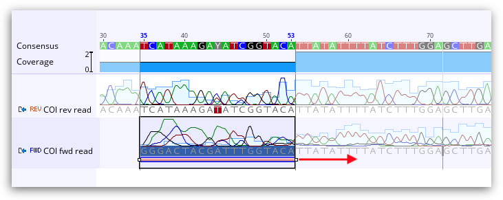
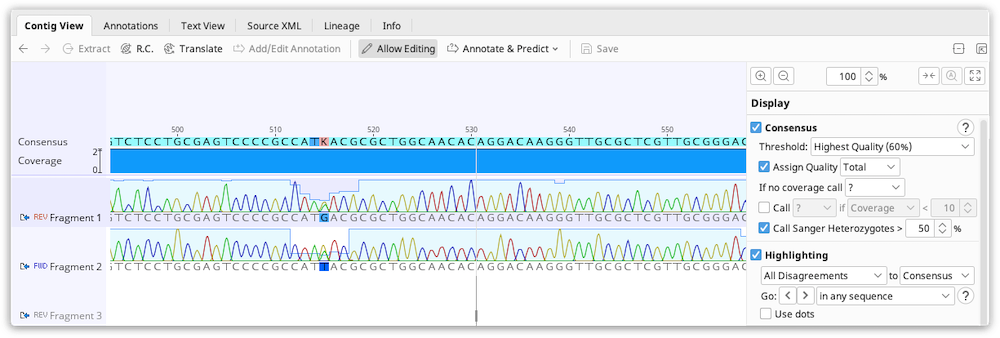
The Contig Viewer
Contigs in Geneious Prime are viewed and edited in exactly the same way as alignments (see Alignment Viewing and Editing). Features particularly relevant to contig assemblies are highlighted on the Figure below:
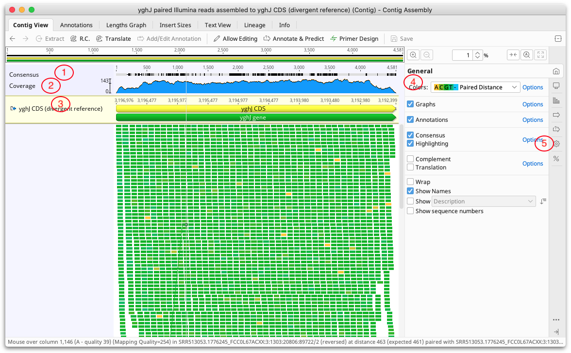
1. Consensus Sequence
The consensus sequence is displayed at the top of the assembly. This is the consensus of the reads only and does not include the reference sequence if one is present. The consensus settings can be found under the Display tab. If the sequences in the contig have quality information attached we recommend selecting the Highest Quality consensus type. In most cases this removes the need for manually editing the contig because the consensus will be the base with the highest total quality at each position.
2. Coverage Graph
The coverage graph shows how many reads map at each position and can be useful for assessing the quality of your mapping. The Graphs tab enables you to show or hide the Coverage graph as well as enable other graphs such as the Identity or Sequence Logo graphs. See Alignment Viewer Graphs for a detailed description of these graphs. The data underlying these graphs can be exported in CSV format by clicking the Export option under the Graphs tab.
3. Reference sequence
If you have run Map to Reference, the reference sequence is shown at the top of the assembly and is shaded yellow.
4. Color schemes
The coloring of bases in the assembly can be selected from the dropdown Colors menu at the top of the General tab. Color schemes particularly useful for contig assemblies include the following:
-
For assemblies of Sanger chromatograms, the default color scheme is Base call quality. This assigns a shade of blue to each base based on its quality. Dark blue for confidence < 20, blue for 20 - 40 and light blue for > 40.
-
For assemblies of paired reads, the default color scheme is Paired Distance. With this color scheme paired reads are colored according to how close the actual separation between the reads is to their expected separation. Green indicates they are correct, yellow and blue indicate under or over their expected separation and red indicates the reads are incorrectly orientated. To configure the colors used, and the sensitivity for deciding if reads are close enough to their expected distance, click the Options link next to the color chooser. The status bar below the viewer will show the actual and expected separation between a particular pair of reads when you hover the mouse over one of the reads in the pair.
-
The Mapping Quality color scheme can be selected for reads mapped to a reference sequence. A mapping quality represents the confidence that the read has been mapped to the correct location. For a read with mapping quality Q, the probability that it has been incorrectly mapped is 10(-Q/10). For example, a read with a mapping quality score of 20 has a 1% chance of having been incorrectly mapped. Reads that could be mapped to multiple locations will have a maximum mapping quality score of 3, which indicates at least a 50% probability of the read mapping elsewhere. Mapping qualities have a maximum value of 254 for consistency with the SAM/BAM format. If a sequence has no mapping quality (i.e the document was produced in a version of Geneious prior to 8.1 or imported from a SAM/BAM file that didn?t have mapping quality) then it will be colored gray. Mapping quality for the sequence under the mouse is also displayed in the status bar. All mappers use heuristics to calculate mapping qualities. For unpaired reads, the Geneious mapper assigns a mapping quality of 20*(the number of additional mismatches in the second best location the read maps to). For paired reads the individual unpaired mapping qualities are calculated, but these are increased by up to 20 depending on how close the best pair is to the expected insert distance compared with the second best pair.
-
The By Direction color scheme allows you to quickly see whether reads are mapped in the forward or reverse orientation.
5. Advanced Layout settings
The settings under the  Advanced tab contain options for adjusting the layout of the contig.
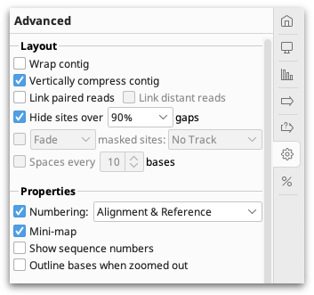
Assemblies of short read data are normally viewed with the option Vertically compress contig enabled. This option puts the reads side by side where possible so that multiple reads can be viewed in the same row. Vertically compress contig cannot be enabled if Wrap contig is switched on. Wrap Contig will wrap the assembly to the screen width and is not recommended for large assemblies.
Hide sites over x % gaps hides sites that have over the set percentage of gaps, so that indels introduced by sequencing errors do not interfere with the viewing of the alignment. This setting does not hide sites where the reference is a non-gap, and does not hide scaffolding gaps in de novo contigs. This setting can only be enabled when wrap contigs is switched off, and editing mode is switched off.
Link Paired Reads: With this option on, pairs of reads will be laid out in the same row with a horizontal line connecting them. This option is only visible on contigs containing reads that have been paired before assembling. Reads separated by more than 3 times their expected distance are not linked by default unless the Link distant reads setting is turned on.
The horizontal line between paired reads is colored according to how close the separation between the reads is to their expected separation. The coloring is the same as for Paired Distance coloring described above, where Green indicates they are correct, yellow and blue indicate under or over their expected separation and red indicates the reads are incorrectly orientated.
If Link Paired Reads is off, it is still possible to view the connecting line between any pair of reads by mousing over one of the reads. To find the pair of a particular read, right click on the read and choose Go to paired mate.
Finding regions of low/high coverage
In addition to the coverage graph which gives you a quick overview of coverage, under the Annotate & Predict toolbar is the Find Low/High Coverage feature. This feature annotates all regions of low/high coverage which you can then navigate through using the little left and right arrows next to the coverage annotations in the controls on the right. You can set the threshold low/high coverage by either specifying an absolute number of sequences or a number of standard deviations from the mean coverage.
The find low/high coverage tool can also be used to record the minimum, mean, and maximum coverage of each annotation of a particular type on the reference sequence. To do this, in the Only Find In section of the options, turn on Annotations in reference sequence of type and choose Create annotations of same type on reference sequence.
Editing Contigs
Editing a contig is exactly the same as editing an alignment in Geneious Prime. After selecting the contig, click the Allow Editing button in the sequence viewer and you can modify, insert and delete characters like in a standard text editor.
Editing of contigs is done to resolve conflicts between fragments before saving the final consensus. Highlighting can be enabled under the Display tab to enable you to quickly scan for and navigate to sites containing disagreements. With editing enabled, you can change bases which you believe are bad calls to be the base which you believe is the correct call. This is often decided by looking at the quality for each of the bases and choosing the higher quality one. Geneious can do this automatically for you if you use the Highest Quality consensus.
Bases in the consensus sequence can also be edited which will update every sequence at the corresponding position to match what is set in the consensus.
You can also manually move a read mapped to a reference sequence to a specific position in the contig. To do this, select the read and right-click, then choose Move read to position.., and enter the position where you want the left-most base in the read to sit.
Extracting the Consensus
Once you are satisfied with a contig you can save the consensus as a new sequence by clicking on the name of the consensus sequence in your contig and clicking the Extract button above the viewer. You can also generate consensus sequences for single or multiple contig documents by selecting the documents and going to Tools → Generate Consensus Sequence.