Building Phylogenetic Trees

Geneious Prime provides inbuilt algorithms for Neighbour-joining (Saitou & Nei 1987) and UPGMA (Mitchener & Sokal 1957) methods of tree reconstruction, which are suitable for preliminary investigation of relationships between newly acquired sequences. For more sophisticated methods of phylogenetic reconstruction such as Maximum Likelihood and Bayesian MCMC, external plugins for specialist software are available. These can be downloaded from the plugins page on our website or within Geneious by going to Plugins under the Tools menu.

Phylogenetic tree representation

A phylogenetic tree describes the evolutionary relationships amongst a set of sequences. They have a few commonly associated terms that are depicted in the figure below:

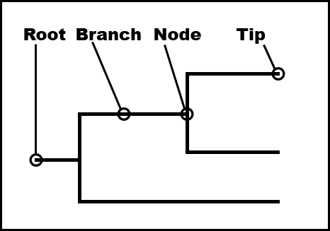
Branch length. A measure of the amount of divergence between two nodes in the tree. Branch lengths are usually expressed in units of substitutions per site of the sequence alignment.

Nodes or internal nodes of a tree represent the inferred common ancestors of the sequences that are grouped under them.

Tips or leaves of a tree represent the sequences used to construct the tree.

Taxonomic units. These can be species, genes or individuals associated with the tips of the tree.

A phylogenetic tree can be rooted or unrooted. A rooted tree consists of a root, or the common ancestor for all the taxonomic units of the tree. An unrooted tree is one that does not show the position of the root. An unrooted tree can be rooted by adding an outgroup (a species that is distantly related to all the taxonomic units in the tree).

For information on viewing and formatting trees in Geneious, see Viewing and Formatting Trees.

Tree building in Geneious Prime

To build a tree, select an alignment or a set of related sequences (all DNA or all protein) in the Document table and click the Tree icon or choose this option from the Tools menu.

If you are building a simple tree (Neigbour joining or UPGMA) using the Geneious tree builder, the tree can be built directly from a set of unaligned sequences, as the alignment will be built as part of the tree-building process. For more advanced trees, or if you wish to bootstrap your trees you must build an alignment first and use that as input for your tree. You can also select an existing tree document (which contains an alignment) and build another tree from that, as the alignment will simply be extracted from the existing tree and used build the new tree.

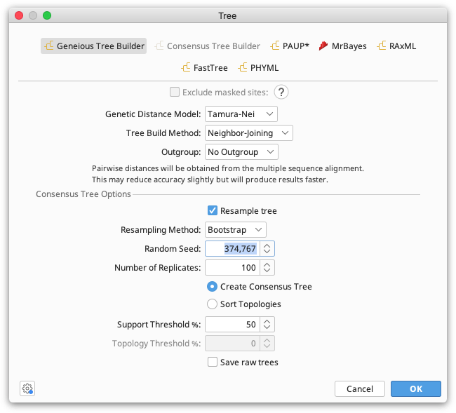
The following options are available in the tree-building dialog for the Geneious tree builder. For more information on these options see Tree building methods and models.

• Exclude masked sites. Excludes sites containing Masked annotations from the analysis without permanently removing them from your alignment. See Using alignment masks for further information.

• Genetic distance model. This lets the user choose the kind of substitution model used to estimate branch lengths. If you are building a tree from DNA sequences you have the choices "Jukes Cantor", "HKY" and "Tamura Nei". If you are building a tree from amino acid sequences you only have the option of "Jukes Cantor" distance correction.

• Tree building method. There are two methods under this option - Neighbor joining and UPGMA.

• Outgroup. Choose which sample to use as an outgroup, or leave it as "no outgroup" to build an unrooted tree.

• Resample tree. Check this to turn on resampling options (bootstrapping or jackknifing) to generate support values for your tree. See Resampling for further information.

• Resampling method. Either bootstrapping or jackknifing can be performed when resampling columns of the sequence alignment.

• Number of samples. The number of alignments and trees to generate while resampling. A value of at least 100 is recommended.

• Create Consensus Tree. Choose this to create a consensus tree from the resampled data.

• Sort Topologies. Produce trees which summarise the topologies resulting from resampling.

• Support threshold. This is used to decide which monophyletic clades to include in the consensus tree, after comparing all the trees in the original set. For example setting this on 50

• Topology Threshold. The percentage of topologies in the original trees which must be represented by the summarizing topologies.

• Save raw trees. If this is turned on then all of the trees created during resampling will be save in the resulting tree document. The number of raw trees saved will therefore be equal to the number of samples.

Using alignment masks

To exclude certain sites or regions of your alignment before tree building, you can apply Masked-type annotations to an alignment's consensus sequence. Masked-type annotations can be applied manually, or using the Mask Alignment option under the Tools menu. This tool enables you to either annotate masked sites, or make a copy of the alignment with masked sites removed. If you choose to annotate masked sites, these can be removed for tree building by checking Exclude masked sites in the Tree building options. With this option, any sites covered by Masked-type annotations will not be used when the tree is inferred but will be retained on the alignment.

Masked-type annotations can be either directly on the consensus sequence of the alignment, or on one or more tracks. If you have multiple tracks containing Masked annotations, you need to select the track you want to use in the Exclude masked sites option. In this way, you can use multiple masks to compare trees inferred from different subsets of your alignments (e.g., excluding different codon positions, or excluding fast-evolving sites). Only the track used to exclude masked sites when inferring the tree will be shown in the Alignment View once the tree is built.

Tree building methods and models

Neighbor-joining

In this method, neighbors are defined as a pair of leaves with one node connecting them. The principle of this method is to find pairs of leaves that minimize the total branch length at each stage of clustering, starting with a star-like tree. The branch lengths and an unrooted tree topology can quickly be obtained by using this method without assuming a molecular clock (see Saitou & Nei 1987).

UPGMA

This clustering method is based on the assumption of a molecular clock. It is appropriate only for a quick and dirty analysis when a rooted tree is needed and the rate of evolution does not vary much across the branches of the tree (see Mitchener & Sokal 1957).

Distance models or molecular evolution models for DNA sequences

The evolutionary distance between two DNA sequences can be determined under the assumption of a particular model of nucleotide substitution. The parameters of the substitution model define a rate matrix that can be used to calculate the probability of evolving from one base to another in a given period of time. This section briefly discusses some of the substitution models available for the Geneious tree builder. Most models are variations of two sets of parameters -- the equilibrium frequencies and relative substitution rates.

Equilibrium frequencies refer to the background probability of each of the four bases A, C, G, T in the DNA sequences. This is represented as a vector of four probabilities πA, πC, πG, πT that sum to 1.

Relative substitution rates define the rate at which each of the transitions (A ↔ G, C ↔ T) and transversions (A ↔ C, A ↔ T, C ↔ G, G ↔ T) occur in an evolving sequence. It is represented as a 4x4 matrix with rates for substitutions from every base to every other base.

Additionally, gaps are not penalized when using the Geneious Tree Builder. Sites with gaps are ignored when calculating pairwise distances (i.e, gaps are not treated as a fifth nucleotide state). Similarly, sites with ambiguous nucleotides are always ignored in distance calculations.

Jukes-Cantor

This is the simplest substitution model. It assumes that all bases have the same equilibrium base frequency, i.e., each nucleotide base occurs with a frequency of 0.25 in DNA sequences. This model also assumes that all nucleotide substitutions occur at equal rates (see Jukes and Cantor 1969).

If the proportion of non-gap, non-ambiguous sites that are mismatched between the sequences is given as p, the formula for computing the distance between the sequences is:

d = -3/4 * log(1 - 4/3 * p)

Under Jukes-Cantor, the number of substitutions is assumed to be Poisson distributed with a rate of 4/3u, i.e. the probability of no substitutions at a given site over a branch of length ut is e^-4/3ut.

HKY

The HKY model assumes every base has a different equilibrium base frequency, and also assumes that transitions evolve at a different rate to the transversions (see Hasegawa et al 1985).

Tamura-Nei

This model also assumes different equilibrium base frequencies. In addition to distinguishing between transitions and transversions, it also allows the two types of transitions (A ↔ G and C ↔ T) to have different rates (see Tamura & Nei 1993).

Distance models or molecular evolution models for Amino Acid sequences

The evolutionary distance between two amino acid sequences can be determined under the assumptions of a particular model of amino acid substitution. The substitution model defines a rate matrix that can be used to calculate the probability of evolving from one amino acid to another over a given time.

As with nucleotides, gaps are not penalized when using the Geneious Tree Builder. Sites with gaps are ignored when calculating pairwise distances (i.e., gaps are not treated as a 21st amino acid state).

Jukes-Cantor

This is the simplest substitution model. It assumes that all amino acids have the same equilibrium base frequency, i.e., each amino acid occurs with a frequency of 0.05 in protein sequences. This model also assumes that all amino acid substitutions occur at equal rates.

If the proportion of non-gap, non-ambiguous sites that are mismatched between the sequences is given as $p$, the formula for computing the distance between the sequences is:

d = -19/20 * log(1 - 20/19 * p)

Under Jukes-Cantor the number of substitutions is assumed to be Poisson distributed with a rate of 20/19u, i.e., the probability of no substitutions at a given site over a branch of length ut is e^-20/19ut.

Technically, Jukes-Cantor for amino acid sequences is the Neyman model (Neyman 1971) with 20 states.

Advanced Tree Building methods

Other plugins are available for running maximum likelihood or Bayesian phylogenetic analyses in Geneious, including MrBayes, PhyML, RAxML, FastTree, and PAUP*. These can be downloaded from the plugins page on our website or within Geneious by going to Plugins under the Tools menu. For more information on running these programs, please consult the user manual for the source software.

Resampling - Bootstrapping and jackknifing

Resampling is a statistical technique where a procedure (such as phylogenetic tree building) is repeated on a series of datasets generated by sampling from one original dataset. The results of analyzing the sampled datasets are then combined to generate summary information about the original dataset.

In the context of tree building, resampling involves generating a series of sequence alignments by sampling columns from the original sequence alignment. Each of these alignments (known as pseudoreplicates) is then used to build an individual phylogenetic tree. A consensus tree can then be constructed by combining information from the set of generated trees or the topologies that occur can be sorted by their frequency (see below).

To resample a tree by bootstrapping or jackknifing with the Geneious Tree Builder, tick Resample Tree under the Consensus Tree Options and choose the method and number of replicates you want to perform.

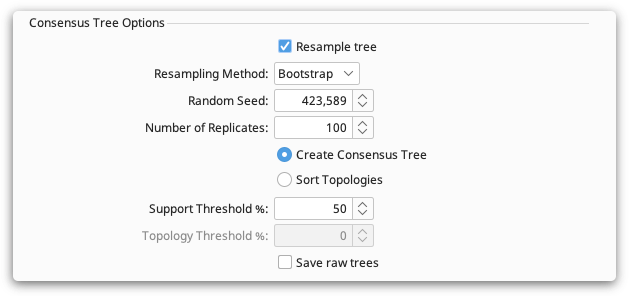
Bootstrapping is the statistical method of resampling with replacement. To apply bootstrapping in the context of tree building, each pseudo-replicate is constructed by randomly sampling columns of the original alignment with replacement until an alignment of the same size is obtained (see Felsenstein 1985).

Jackknifing is a statistical method of numerical resampling based on deleting a portion of the original observations for each pseudo-replicate. A 50% jackknife randomly deletes half of the columns from the alignment to create each pseudo-replicate.

Consensus trees

A consensus tree provides an estimate for the level of support for each clade in the final tree. It is built by combining clades which occurred in at least a certain percentage of the resampled trees. This percentage is called the consensus support threshold. A 100% support threshold results in a Strict consensus tree which is a tree where the included clades are those that are present in all the trees of the original set. A 50% threshold results in a Majority rule consensus tree that includes only those clades that are present in the majority of the trees in the original set. A threshold less that 50% gives rise to a Greedy consensus tree. In constructing a Greedy consensus tree clades are first ordered according to the number of times they appear (i.e. the amount of support they have), then the consensus tree is constructed progressively to include all those clades whose support is above the threshold and that are compatible with the tree constructed so far.

The length of the consensus tree branches is computed from the average over all trees containing the clade. The lengths of tip branches are computed by averaging over all trees.

Note: The above definitions apply to rooted trees. The same principles can be applied to unrooted trees by replacing "clades" with "splits". Each branch (edge) in an unrooted tree corresponds to a different split of the taxa that label the leaves of this tree.

Creating a consensus tree of existing trees

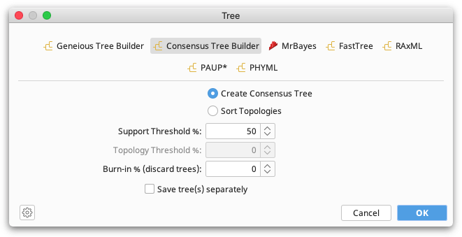
Select a tree set document (e.g. a set of bootstrap replicate trees) and choose Tree then Consensus Tree Builder at the top of the setup dialog. Check Create Consensus Tree and choose the Support Threshold % you wish to use. This will create a consensus tree using the trees already in the document (no resampling will be performed) and it will either be added to the tree document or saved as a separate tree document.

Sort topologies

This will produce one or more trees sorted by topology, summarizing the results of resampling, check Sort topologies under the Consensus Tree Builder options. The frequency of each topology in the set of original trees is calculated and the topologies are sorted by their frequency. A number of these topologies, based on the topology threshold, will be output as summary trees. The summary trees have branch lengths that are the average of the lengths of the same branch from trees with the same topology.

The topology threshold determines what percentage of the original tree topologies must be represented by the summarizing topologies. The most common topology will always be output as the first summary tree. If the frequency (%) of this does not meet the threshold then the next most frequent topology will be added, and so on until the total frequency of the topologies reaches the threshold value.

A topology threshold of 0 will result in only the most common topology being output, a threshold of 100 will result in all topologies being output.

Viewing and formatting trees

Once the tree is built it will appear in the Document Viewer window.

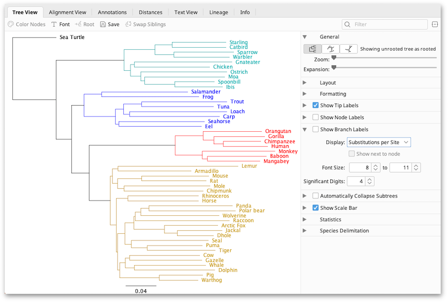
When viewing a tree a number of other view tabs may be available depending on the information at hand. The Alignment View tab will be visible if the tree was built from a sequence alignment using Geneious. The Text View shows the tree in text format (Newick).

The tabs to the right of the tree viewer contain options for controlling the look of the tree, and the information displayed on it. The toolbar above the tree provides additional formatting options, and allows you to change the root, or rearrange the tree. The subsequent sections provide more detail on these options.

Current Tree

If you are viewing a tree set, this option will be displayed. Select the tree you want to view from the list.

General

The General tab has 3 buttons showing the different possible tree views: rooted, circular, and unrooted. The Zoom slider controls the zoom level of the tree while the Expansion slider expands the tree vertically (in the rooted layout).

Layout

This has different options depending on the layout that you select above:

• Root Length Sets the length of the visible root of the tree (Rooted and Circular trees)

• Curvature Adds curvature to the tree branches (Rooted view only)

• Align Taxon Labels Aligns the tip labels to make viewing a large tree easier (Rooted view only)

• Root Angle Rotates the tree in the viewer (Circular and Unrooted views)

• Angle Range Compresses the branches into an arc (Circular view only)

Formatting

The following options are available for formatting branches:

• Flip the tree horizontally flips the tree so that branches go from right to left, rather than left to right.

• Transform branches allows the branches to be equal like a cladogram, or proportional. Leaving it unselected leaves the tree in its original form.

• Ordering orders branches in increasing or decreasing order of length, but within each clade or cluster.

• Show root branch displays the position of the root of the tree (has no effect in the unrooted layout).

• Line weight can be increased or decreased to change the thickness of the lines representing the branches.

• Show selected subtree only shows only the part of the tree that is selected (or the entire tree if there is no selection).

Show Tips, Node and Branch Labels

Show tip labels: This refers to labels on the tips of the branches of the tree. Tip labels can be any of the fields on your document, and can be set in the Display option. To select multiple fields to display at the tips, hold down the command/control key while selecting.

Show node labels: This refers to labels on the internal nodes of the tree. If you are viewing a consensus tree, you can display consensus support % here, or you can display the node heights.

Show branch labels: This refers to labels the branches of the tree. You can display substitutions per site (branch lengths) here, or for a consensus or bootstrapped tree you can display consensus support % or bootstrap support %. Checking "show next to node" will move the labels from the middle of the branch to adjacent to the node.

For node and branch labels, the font can be set using the Font Size options in the tab. The tree viewer will shrink the font size of some labels if they cannot all fit in the available space. The lower end of the range specifies the minimum size that the tree viewer is allowed to shrink the label font to. The font sizes for the tip labels are set using the Font button in the toolbar above the tree viewer. Significant Digits sets how many digits to display if the value the node is displaying is numeric.

Automatically collapse subtrees

This option enables groups of similar nodes to be collapsed into a single node that represents that subtree. The maximum distance within the subtrees is determined by the Subtree Distance slider. Use this option to help navigate trees with many nodes and tips.

Collapsed nodes are labelled with the name of one of the tips, a count of how many tips the subtree contains, and the maximum distance between the top of the subtree and any of the tips within it. Double-clicking a node in a tree will force it to expand or contract. Automatically Collapse Subtrees will not override this state. To reset the state of double-clicked nodes in the tree, click Reset state of X nodes. X is the number of nodes with a manually expanded or collapsed state.

Show scale bar

This displays a scale bar at the bottom of the tree view to indicate the length of the branches of the tree. It has three options: Scale range, font size and line weight. Setting the scale range to 0.0 allows the scale bar to choose its own length, otherwise it will be the length that you specify.

Statistics

Displays information on the number of nodes and number of tips in the tree.

The Toolbar

The buttons on the toolbar along the top of the viewer allow you to edit the tree.

Click on a node in the tree viewer to select the node and its clade. Double-click the node to collapse/un-collapse the clade in the view. Once you have selected a clade in the view, you can edit it using the following toolbar buttons:

• Color Nodes: allows you to choose a new color for the selected clade.

• Font: allows you to change the font for the tip labels.

• Root: allows you to re-root the tree on the selected node.

• Swap Siblings: allows you to swap the position of the sibling clades of the selected node.

The toolbar also contains a Search box that allows you to search for particular tip labels. If a match is found, this tip is displayed on the tree and all other tips are greyed out. If you wish to search by a field that is not currently displayed on a tip label, you need to change the field under Show Tip Labels first.